Home / Semantic Search Algorithms: The Models and Methods Behind Them

Semantic Search Algorithms: The Models and Methods Behind Them

Semantic search algorithms fall into two layers: representation algorithms that turn text into something comparable by meaning, and search algorithms that find the closest matches quickly. The representation layer has evolved from lexical weighting such as TF-IDF and BM25, through latent semantic indexing, to neural embeddings. Today’s main families are dense retrieval with bi-encoders, learned sparse retrieval such as SPLADE, and late interaction such as ColBERT. Cross-encoders rerank the top results. The search layer uses approximate nearest neighbour algorithms, such as HNSW graphs, IVF clustering, product quantization and locality-sensitive hashing. They avoid comparing a query with every vector. Most production systems combine several: BM25 plus dense retrieval in hybrid search, an HNSW index for speed, and a reranker for precision. There is no single best algorithm; the right mix depends on data, queries and budget.

What are semantic search algorithms?

Semantic search algorithms are the methods that represent queries and documents by meaning and retrieve the documents closest to a query. They span models that create representations and data structures that search them.

Two questions define any semantic search system. First, how is meaning represented, so that “car insurance claim” and “filing a claim after an accident” count as close? Second, how are the closest documents found among millions without comparing each one? The first is answered by representation algorithms, the second by index or similarity search algorithms. How semantic search works shows how the two fit together.

The field grew out of information retrieval, covered in what is information retrieval. Many older algorithms are still in use, often alongside newer ones, because each family has strengths the others lack. Knowing the families makes it easier to read product documentation and research papers.

How have semantic search algorithms changed over time?

Semantic search algorithms have changed from word-counting methods in the 1970s, through latent semantic models around 1990, to neural embeddings from 2013 and transformer-based retrieval from 2019. Each step captured more meaning.

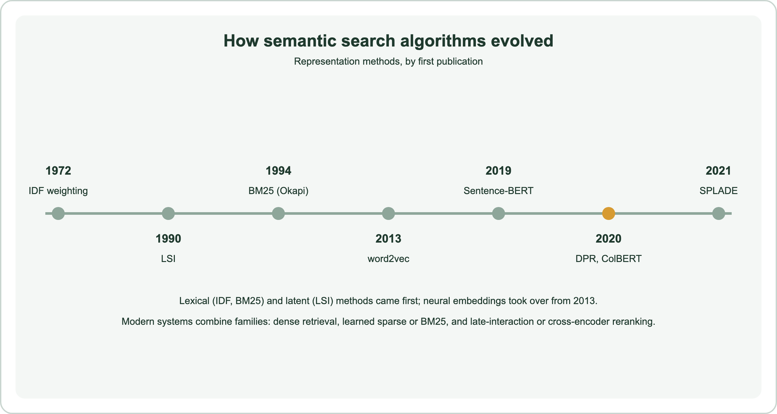
Karen Spärck Jones introduced inverse document frequency in 1972, the idea that rare words carry more information. BM25, from Robertson and colleagues in the Okapi system and presented at TREC in 1994, refined term weighting and is still a standard baseline. Latent semantic indexing, from Deerwester and colleagues in 1990, compressed word-document counts into a smaller space where related words cluster. That was an early form of semantic matching, covered in latent semantic indexing.

Neural methods followed. Word2vec, from Mikolov and colleagues in 2013, learned dense word vectors, covered in word2vec and GloVe. Transformers and BERT brought context-aware representations, and Sentence-BERT in 2019 made them practical for search, as covered in Sentence-BERT. Dense passage retrieval and ColBERT arrived in 2020, and SPLADE in 2021.

What are the main families of semantic search algorithms today?

The main families of semantic search algorithms today are dense retrieval, learned sparse retrieval, late interaction and cross-encoder reranking, usually combined with BM25. They differ in how they represent text and what they cost.

Dense retrieval uses a bi-encoder to turn each text into one vector of a few hundred numbers and compares vectors by cosine similarity. It handles paraphrases well and scales to large collections, as covered in dense retrieval. Learned sparse retrieval, such as SPLADE from Formal and colleagues in 2021, produces weighted vocabulary terms that an inverted index can search. It keeps the precision of keywords while adding related terms; see SPLADE and learned sparse retrieval.

Late interaction, introduced by ColBERT, keeps a vector per token and matches tokens individually. That gives finer matching at higher storage cost, covered in ColBERT and late interaction. Cross-encoders read the query and a document together and score their relevance directly. They are the most accurate but slowest, so they rerank a shortlist, as covered in cross-encoders. Retrieval models explained compares all of them.

Why do lexical algorithms like BM25 still matter?

Lexical algorithms like BM25 still matter because they match exact words reliably, need no training, and often beat neural models on unfamiliar domains, rare names and codes. They complement semantic methods rather than compete with them.

BM25 scores documents by how often query terms appear, how rare those terms are, and how long the document is. It finds product codes, error messages and proper names that embeddings can blur. The BEIR benchmark showed BM25 to be a strong baseline across many domains, and several dense models trained on one dataset did not beat it everywhere. The BM25 algorithm and TF-IDF explain the formulas.

Lexical search fails on vocabulary mismatch, when the query and the document use different words for the same thing. That gap is what semantic algorithms fill, as described in the vocabulary mismatch problem. Combining the two in hybrid search covers both failure modes.

What is the best similarity search algorithm?

There is no single best similarity search algorithm, but HNSW is the most common default for vector search because it gives fast queries with high recall and supports updates. IVF and product quantization suit memory-bound cases.

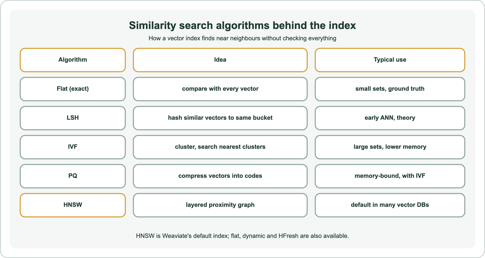
Exact search compares a query with every vector and is the reference for accuracy, as covered in exact vs approximate search. Locality-sensitive hashing, from Indyk and Motwani in 1998, hashes similar vectors into the same buckets. IVF clusters vectors and searches only the clusters nearest the query. Product quantization, from Jégou and colleagues in 2011, compresses vectors into short codes for fast approximate distances.

HNSW, from Malkov and Yashunin, builds a layered graph that a query walks towards its nearest neighbours. It is Weaviate’s default vector index, and Weaviate also offers flat, dynamic and HFresh indexes for other trade-offs. The best choice depends on collection size, memory budget, update rate and recall target. Approximate nearest neighbor search covers the algorithms in depth.

How do the algorithm families compare on cost?

The algorithm families compare on cost mainly through when the model runs and how much they store: bi-encoders and sparse models run once per document, while cross-encoders run once per query-document pair. Storage grows with vectors per document.

BM25 needs no model and stores an inverted index, so it is the cheapest to run. Dense retrieval embeds every document once at import and every query at search time, then stores one vector per document, so memory scales with collection size times vector length. Learned sparse models also run once per document but store weighted terms in an inverted index. Late interaction stores one vector per token, which multiplies storage, as covered in multi-vector search.

Cross-encoders store nothing extra but run the model for every candidate at query time, which is why they only rerank a shortlist. Compression and smaller models lower the cost of every family, and the comparison in bi-encoder vs cross-encoder shows where the line usually falls.

How do production systems combine semantic search algorithms?

Production systems combine these algorithms in stages: fast first-stage retrieval with dense and lexical methods, fusion of their results, and slower reranking of a shortlist. Each stage uses the algorithm that fits its cost budget.

A typical pipeline embeds the query with a bi-encoder, searches an HNSW index, runs BM25 on the same collection, and fuses the two lists. A cross-encoder then reranks the top few dozen results. In Weaviate, a hybrid query performs the first three steps, and a reranker integration adds the fourth. How hybrid search works and what is reranking cover the stages.

Query-side algorithms add another layer. Query rewriting and expansion change the query before retrieval, covered in query understanding. Agentic retrieval lets a language model plan several searches, covered in agentic retrieval and agentic search. These sit on top of the same core algorithms.

How do you choose semantic search algorithms for a project?

You choose semantic search algorithms by starting with a strong default, hybrid dense plus BM25 on an HNSW index, then measuring on your own queries and adding complexity only where it helps. Evaluation decides, not novelty.

Begin with an embedding model chosen for your language and domain, as covered in what are embeddings, and hybrid search for exact terms. Measure recall and nDCG on judged queries using the methods in how to evaluate semantic search and information retrieval metrics. Add a reranker if precision at the top falls short, learned sparse retrieval if exact terms still fail, or late interaction if fine matching matters and storage allows.

Weigh cost and scale alongside quality. Each added stage adds latency and infrastructure, as covered in scaling semantic search. Tools and databases differ in which algorithms they support, compared in semantic search tools compared. For background, see what is semantic search and how to build semantic search.

Semantic search algorithms have two layers. Representation algorithms, from TF-IDF and BM25 through latent semantic indexing to neural dense, learned sparse and late-interaction models, decide what counts as similar. Similarity search algorithms, such as HNSW, IVF, product quantization and LSH, find similar items quickly without checking everything. HNSW is the common default index, and BM25 remains a strong partner in hybrid search. Production systems combine fast retrieval, fusion and reranking. Start with hybrid dense plus BM25, measure on real queries, and add stages only where they help.