Home / How it works / How Semantic Search Works, Step by Step
How Semantic Search Works, Step by Step
Semantic search works by turning content and queries into comparable representations, then retrieving and ranking the stored items whose representations sit closest to the query. The work splits into two paths. An offline path chunks documents, embeds them, stores metadata, and builds an index before anyone searches. An online path embeds each query, finds nearby candidates in that index, applies filters, and orders the results. Each stage makes its own decision: what unit can be returned, which model defines closeness, which metric measures it, and how many candidates survive. Search quality comes from all of those decisions together, so a failure is diagnosed by finding the stage that lost the relevant item.
Semantic search in four facts
- Semantic search prepares content offline and answers each query through a separate online path.
- The distance metric should match the metric used to train the embedding model.
- A nearest-neighbor search always returns a closest result, even when no stored item is relevant.
- Reranking can reorder retrieved candidates but cannot add an item that retrieval missed.
What does semantic search match that keyword search can miss?
Semantic search matches related meaning, so it can connect paraphrases and differently worded text that share few exact tokens. A query such as How can I reduce RAM use? may need a chunk titled Diagnosing memory leaks. The two strings share almost no words, yet they describe the same problem. The pair is illustrative, not a measured result.
Keyword search compares analyzed tokens, so it needs some literal overlap. Semantic retrieval compares learned representations instead, which is why semantic matching can bridge wording that a token index cannot. Synonyms and related terms are the most familiar case of this vocabulary mismatch, but conversational questions and descriptions of symptoms create it too.
Weaviate’s vector search documentation notes that this kind of search is often called semantic search, and that the same mechanism also applies to images, video, and audio. The meaning lives in the model, not in the database. Language coverage follows the same rule. Multilingual and cross-lingual semantic search works only when the configured embedding model aligns several languages in one space. Weaviate lists multilingual models separately from English-only models for that reason.
Literal matching still matters. Weaviate’s keyword search documentation recommends exact token matching for technical terms, precise categories, and tags. Semantic search adds a different kind of evidence rather than replacing lexical evidence. Seeing where that evidence comes from requires following a query through the whole system.
How does semantic search turn a query into ranked results?
Semantic search turns a query into ranked results through an offline ingestion path that prepares content and an online query path that embeds, retrieves, filters, and ranks. The offline path runs before any user searches. The online path repeats for every query. A full semantic search architecture keeps those two paths as separate services because they scale and fail differently.
The complete sequence has eight steps:
- Chunk source documents into the units the system can return.
- Embed each chunk with the chosen model.
- Store each vector with its metadata and a link to its source.
- Index the vectors so nearby items can be found quickly.
- Embed the incoming query with a compatible model.
- Retrieve the nearest candidates from the index.
- Constrain those candidates with filters, a cutoff, or keyword evidence.
- Rank the survivors and return the final list.
Steps one to four belong to ingestion. Steps five to eight belong to the query path. Weaviate’s documentation describes the query side directly: it compares stored object vectors with the query vector and returns the closest results. A query vector can be supplied directly with nearVector, taken from a stored object with nearObject, or generated from text with nearText when a vectorizer is configured.
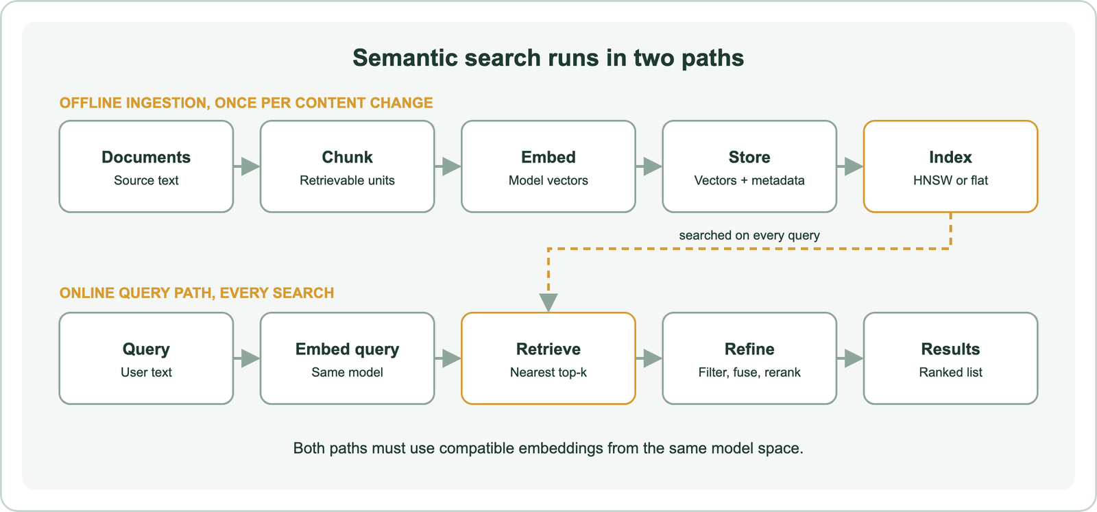
In the running example, the memory-leak chunk is embedded during ingestion and the RAM question is embedded at query time. Whether they meet depends first on how the chunk was prepared.
How does offline ingestion prepare content for semantic search?
Offline ingestion prepares content for semantic search by choosing the retrievable unit, embedding selected fields, storing metadata, and building an index before any query arrives. Every later stage inherits these choices. A query cannot retrieve a sentence that ingestion merged into an unrelated block or dropped entirely.
Chunking for semantic search decides that unit. A chunk that is too large blends several topics into one vector. A chunk that is too small loses the context that makes it meaningful. Weaviate’s retrieval-augmented generation guide states that no chunking strategy fits every case. It offers 100 to 200 words with a 50-word overlap as a starting baseline and recommends linking each chunk back to its source document.
Field selection matters as much as boundaries. By default, Weaviate vectorizes the collection name and text property values, and source properties can restrict which fields enter the embedding. Embedding an SKU field or a boilerplate footer adds noise to the vector. Metadata such as product, date, or permission stays in the object for filtering and display instead.
Ingestion ends with indexing. Semantic indexing and vector indexes turn stored vectors into a structure that the query path can search. Weaviate recommends server-side batching as the starting point for most bulk imports, and objects can carry vectors made elsewhere. Changing the model later means re-embedding every stored item, because old and new vectors do not share one space. That shared space is what the embedding model provides.
How do embeddings make semantic matching possible?
Embeddings make semantic matching possible by mapping queries and content into one vector space where a chosen metric can compare them. An embedding is a list of numbers produced by a trained model. Items the model learned to treat as related land near each other. Items it learned to separate land farther apart.
The geometry comes from training, not from human understanding. Reimers and Gurevych’s 2019 Sentence-BERT paper trained siamese and triplet networks so that sentence embeddings could be compared with cosine similarity. Karpukhin and colleagues’ 2020 Dense Passage Retrieval paper trained a dual encoder, one for questions and one for passages, and retrieved with maximum inner product search. Both designs place queries and documents in a shared space on purpose.
Most text embedding models produce dense vectors. Elastic’s vector search documentation describes them as fixed-length arrays where every element holds a value. Learned term-weight models and lexical encoders can produce sparse vectors instead, where most elements are zero. The dense versus sparse vectors choice decides whether retrieval keeps word-level evidence or compresses meaning into every dimension.
Compatibility is the practical rule. The query must be embedded by the same model that embedded the content, or by a paired encoder trained for that space. A query vector from one model is meaningless against an index built by another. Once compatible vectors exist, the system still has to find the closest ones quickly.
How does a vector index retrieve candidates without scanning everything?
A vector index retrieves candidates without scanning everything by organizing stored vectors so the nearest ones can be reached through a small number of comparisons. Weaviate’s documentation describes the index as balancing recall, throughput, and resource use. Weaviate offers HNSW, flat, and dynamic index types.
Three related terms name different layers. Vector search is the database operation that compares a query vector with stored vectors. Similarity search is the broader task of finding close representations, whatever the data type. Semantic search is the whole system that uses those operations to serve meaning-based queries.
A flat index compares the query with every stored vector, which gives exact results at a cost that grows with the collection. Approximate nearest neighbor search reduces that work by accepting that a few true neighbors may be skipped. Malkov and Yashunin’s 2016 HNSW paper builds a multilayer hierarchy of proximity graphs. A search starts in a sparse upper layer and descends through finer layers toward the query’s neighborhood.
Weaviate’s indexing documentation states the trade directly: its HNSW index offers faster similarity search in exchange for some accuracy compared with exhaustive search. The exact versus approximate search decision therefore balances recall against latency and memory. Whichever index runs, it needs a rule for what “near” means.
How do distance metrics and top-k rules turn proximity into candidates?
Distance metrics and top-k rules turn proximity into candidates by scoring how far each stored vector sits from the query and keeping only the closest items. In Weaviate’s convention, a smaller distance always means greater similarity. Weaviate’s documentation also says the search metric should match the metric used to train the model, and its default is cosine distance.
Cosine, dot product, and Euclidean distance measure different geometry. Weaviate defines cosine distance as one minus cosine similarity, dot distance as the negative dot product, and squared Euclidean distance as the sum of squared differences. Two unit vectors at right angles show the difference:
| Measure | Formula | Value |
|---|---|---|
| Cosine similarity | dot(a, b) / (|a| |b|) | 0 |
| Cosine distance | 1 − cosine similarity | 1 |
| Dot product | 1 × 0 + 0 × 1 | 0 |
| Squared Euclidean distance | (1 − 0)² + (0 − 1)² | 2 |
The same pair gets different numbers under each metric, so scores are only comparable within one configuration. Relevance scores need that context before anyone sets a threshold on them.
Top-k retrieval keeps a fixed number of nearest items. Weaviate’s documentation warns that a nearest-neighbor search always has a closest result, even when nothing is a good match. Limits, AutoCut, a distance threshold, and filters can each trim that list. A count of ten is not proof of ten relevant items, which is why later stages refine the candidates.
How do filters, hybrid retrieval, and reranking refine candidates?
Filters, hybrid retrieval, and reranking refine candidates in different ways: filters restrict eligibility, hybrid retrieval adds lexical evidence, and reranking reorders the shortlist with a stronger model. Each stage works on what the previous stage passed along. None of them can create a candidate from nothing.
Filters come first in Weaviate. Its filtering documentation describes pre-filtering: the inverted index builds an allow-list of eligible IDs before the HNSW search, so only permitted objects can enter results. A product or permission filter therefore shapes the candidate set rather than trimming a finished list.
Pure vector retrieval can blur literal identifiers such as error codes. Hybrid search addresses that gap. Weaviate’s hybrid documentation says it runs vector and BM25 searches in parallel, then normalizes and fuses the two result sets into one ranking. Its alpha parameter runs from 0, keyword only, to 1, vector only. Keyword search remains the better tool when an exact token must appear.
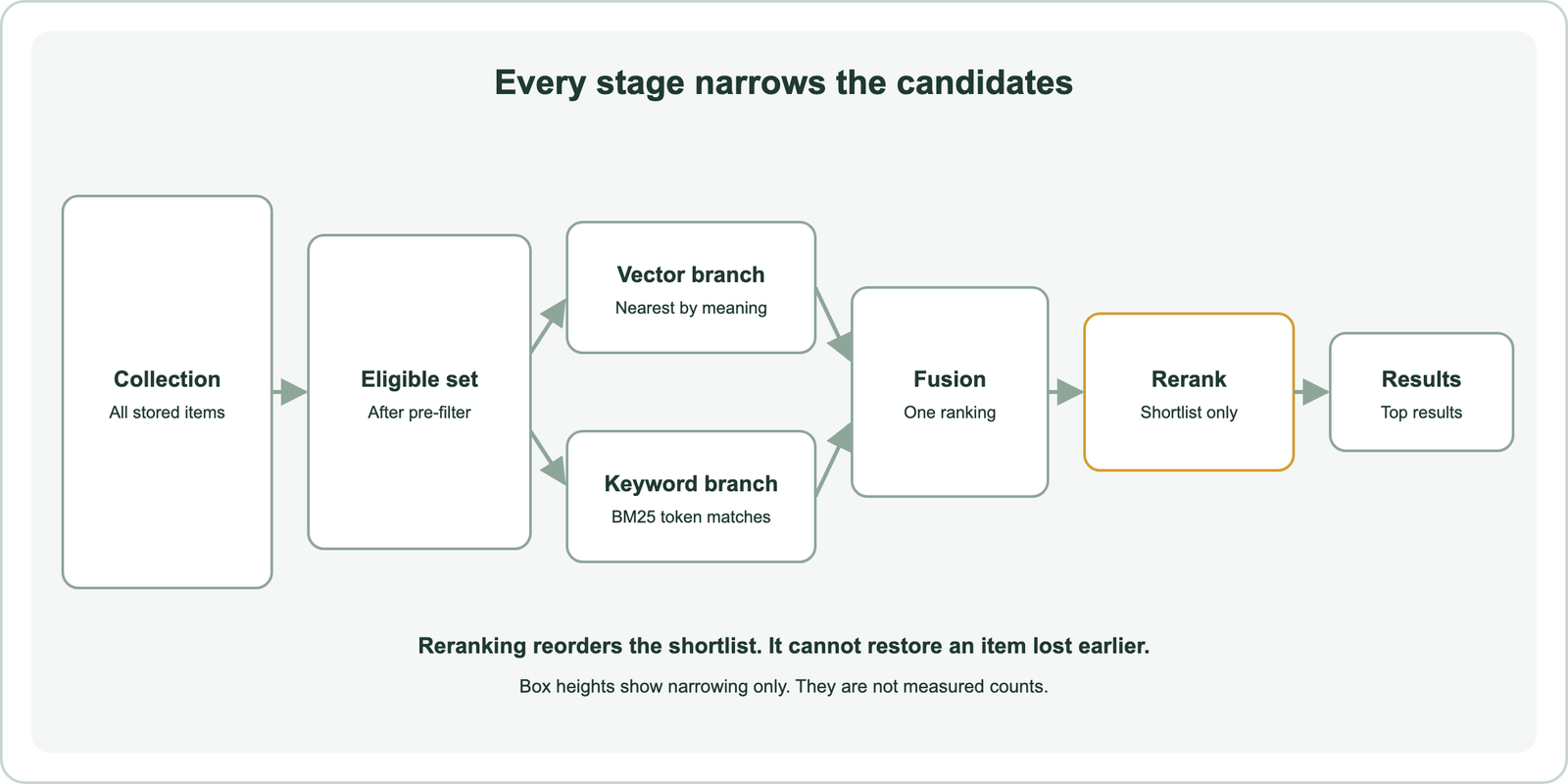
Reranking scores each query and candidate pair with a heavier model. Weaviate’s reranking documentation explains why it runs last: applying an expensive model to every object is usually prohibitive. Weaviate’s search documentation adds that rerank and boost only reorder first-stage results. Because each stage depends on the last, failures need to be traced stage by stage.
Where does semantic search fail, and how should each stage be evaluated?
Semantic search fails at specific stages, so each failure is evaluated by testing the stage that lost or misranked the relevant item. A wrong answer at the end can start with a bad chunk, a mismatched model, a strict filter, or an index that skipped a neighbor. The symptom alone rarely names the cause.
The common failures map to stages like this:
| Stage | Visible symptom | Test | Likely correction |
|---|---|---|---|
| Chunking | Answer split across two results | Read the retrieved chunks | Change boundaries or overlap |
| Field selection | Boilerplate pages rank high | Inspect embedded properties | Embed only meaningful fields |
| Model | Domain terms retrieve generic text | Compare models on judged queries | Choose a domain-suited model |
| Metric | Ordering looks random | Check the model’s training metric | Match the index metric |
| Index | Known neighbor missing | Run exact search on a sample | Tune or change the index |
| Cutoff | Relevant item just below the list | Raise k on judged queries | Adjust k or the threshold |
| Filter | No results for valid queries | Rerun without the filter | Fix metadata or filter logic |
| Exact identifiers | Error codes return near misses | Query the code alone | Add keyword or hybrid retrieval |
The table turns vague complaints into tests. Evaluation then needs a judged query set. The NIST TREC overview defines precision as relevant retrieved items divided by retrieved items, and recall as relevant retrieved items divided by all relevant items. A cutoff such as ten scores only the top ten results. Recall at k shows whether candidates survive retrieval, while precision at k shows whether the returned list is clean.
Change one stage at a time and record latency and memory beside quality. Running exact search on a sample isolates how much recall the approximate index costs. That discipline turns tuning into measurement rather than guesswork.
Semantic search works when content and queries share a useful representation, retrieval keeps enough relevant candidates, and ranking matches the product’s definition of relevance. The offline path decides what can be found: chunks, embedded fields, vectors, and the index. The online path decides what is found: the query embedding, the metric, the cutoff, filters, fusion, and reranking. Proximity alone proves nothing, because a nearest result always exists. The practical decision is to test chunking, model, metric, index, cutoff, and refinement against judged queries, one stage at a time, and keep the configuration that measurably returns the right items.