Home / How it works / What Is Similarity Search and How Does It Power Semantic Retrieval?
ExplainerWhat Is Similarity Search and How Does It Power Semantic Retrieval?
Similarity search is a retrieval method that finds the items in a collection closest to a query, by turning both into vectors and measuring the distance between them. It is the mechanism underneath semantic search, recommendations, image lookup, and retrieval for RAG. In a vector database such as Weaviate, the query is embedded, compared with stored embeddings using a distance metric such as cosine, and the nearest items come back ranked. For small collections the system can compare the query with every item. For large ones it uses an approximate index such as HNSW, which trades a little accuracy for a large gain in speed. The nearest result is not always a relevant one, so practical systems add limits, thresholds, and filters.
Similarity search in four facts
- Similarity search ranks items by vector distance to a query, not by shared words.
- Weaviate supports five metrics: cosine (the default), dot, l2-squared, hamming, and manhattan.
- Flat indexes compare every item; HNSW indexes search approximately in logarithmic time.
- Every vector is near something, so thresholds and autocut stop irrelevant results.
What is similarity search?
Similarity search is the task of finding the items in a dataset that are most like a given query item, where likeness is measured as closeness between numeric representations. It is also called nearest neighbor search, because the answer is the set of points nearest the query.
The idea is older than modern AI. Researchers studied similarity search in metric spaces long before embeddings, including hashing methods published in 1999. What changed is the representation. Embedding models now turn text, images, and audio into vectors that capture meaning, so “finding similar items” works for concepts, not only exact patterns.
In current systems the term almost always means vector similarity search. Each item is stored as an embedding, a list of numbers produced by a model. The query is embedded the same way. The system then returns the stored vectors that sit closest to the query vector. The embeddings guide explains how those vectors are made.
Weaviate’s own concept page describes vector search in exactly these terms. It compares the query’s embedding with stored embeddings using a predefined distance metric and returns the closest matches. Its example shows why this matters: a search for “very dark,” “noir,” or “ebony” still returns a black bear and a black cat, though none of those words appear in the data. The process behind that result has a few distinct steps.
How does similarity search work?
Similarity search works in four steps: embed the items, index the vectors, embed the query, and rank stored vectors by their distance to the query. Similarity search generally relies on three parts: an embedding model, a distance metric, and an index.
- Embed each item with a model, so every document, image, or product becomes a vector.
- Index the vectors in a structure built for fast nearest neighbor lookup.
- Embed the query with the same model, so it lands in the same vector space.
- Rank stored vectors by distance to the query and return the closest ones.
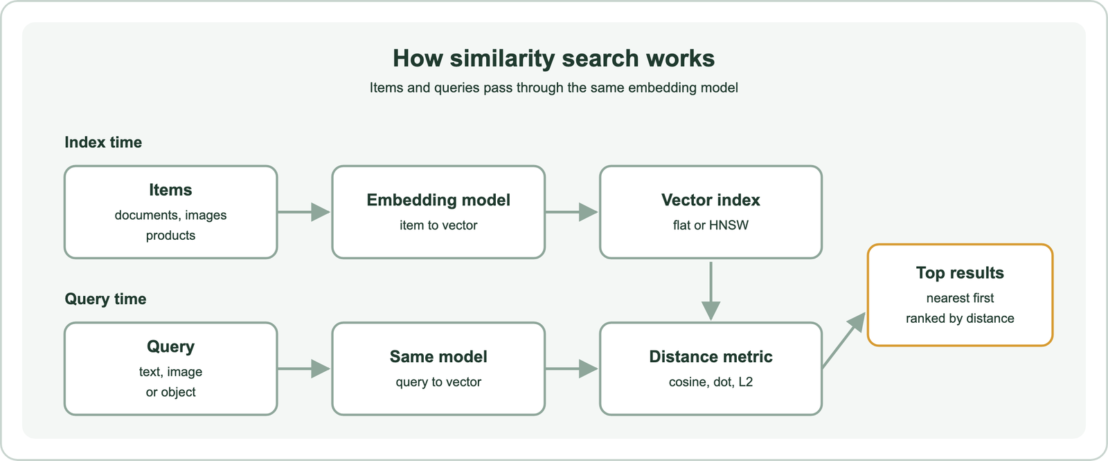
The same model must embed both sides. Vectors from different models live in different spaces, so distances between them mean nothing. In Weaviate, a collection with a configured vectorizer handles this automatically. A nearText query is embedded by the collection’s model before the search runs.
Weaviate offers several ways to supply the query. A nearVector query passes a vector directly. A nearObject query reuses the vector of an existing object, which is how “more like this” features work. A nearText, nearImage, or nearVideo query sends raw input for the model to embed. The guide to how semantic search works places these steps in a full search system. The distance metric in step four deserves its own look.
Which metrics does similarity search use to measure closeness?
Similarity search uses distance metrics such as cosine distance, dot product, squared Euclidean distance, Manhattan distance, and Hamming distance to measure how close two vectors are. In geometric terms, each metric defines what “near” means in the vector space.
| Metric | What it measures | Range | Typical use |
|---|---|---|---|
cosine (default) | Angle between vectors, as 1 minus cosine similarity | 0 (identical) to 2 (opposite) | Most text embedding models |
dot | Negative dot product, so smaller means closer | Unbounded | Models trained for dot product |
l2-squared | Squared straight-line distance | 0 upward | Models trained on Euclidean distance |
manhattan | Sum of absolute differences per dimension | 0 upward | Grid-like or tabular features |
hamming | Count of dimensions that differ | 0 to the dimension count | Binary codes and hashes |
In every Weaviate metric a smaller distance means a closer match. That is why Weaviate reports the dot product as a negative number. When cosine is chosen, Weaviate normalizes vectors and computes a dot product internally, because the result is the same and the calculation is faster.
The right metric is usually not a free choice. Weaviate’s guidance is to use the metric the embedding model was trained with, which the model’s documentation normally states. Other metrics exist, such as Jaccard similarity for sets and Chebyshev distance for maximum coordinate difference. These matter for specialized data but rarely for embeddings.
Metrics also drive cost. Weaviate’s documentation notes that in a typical deployment, most CPU time goes into calculating vector distances, which is why it uses SIMD instructions for cosine, dot, and l2-squared. The comparison of cosine, dot product, and Euclidean distance covers the math. Cost is also why most systems avoid comparing the query with everything.
Does similarity search compare the query with every item?
Similarity search compares the query with every item only in exact, or brute-force, search; large systems use approximate nearest neighbor indexes that check a small fraction of items. The choice depends mainly on collection size.
Exact search, often called k-nearest neighbors or k-NN, computes the distance from the query to every stored vector and keeps the closest k. The results are guaranteed correct, but the work grows in a straight line with the number of items. Weaviate’s flat index works this way. Its documentation describes the flat index as having linear time complexity, a very small memory footprint, and a good fit for small collections.
Approximate nearest neighbor search, or ANN, gives up the guarantee to gain speed. Weaviate’s default index is HNSW, the graph method published by Malkov and Yashunin. It builds layers of linked vectors and walks from coarse to fine layers toward the query. Weaviate describes its query time as logarithmic. As Weaviate’s engineering blog puts it, the index does not look for the exact closest vectors, so recall becomes the measure of quality, and the recall and latency trade-off can be tuned.
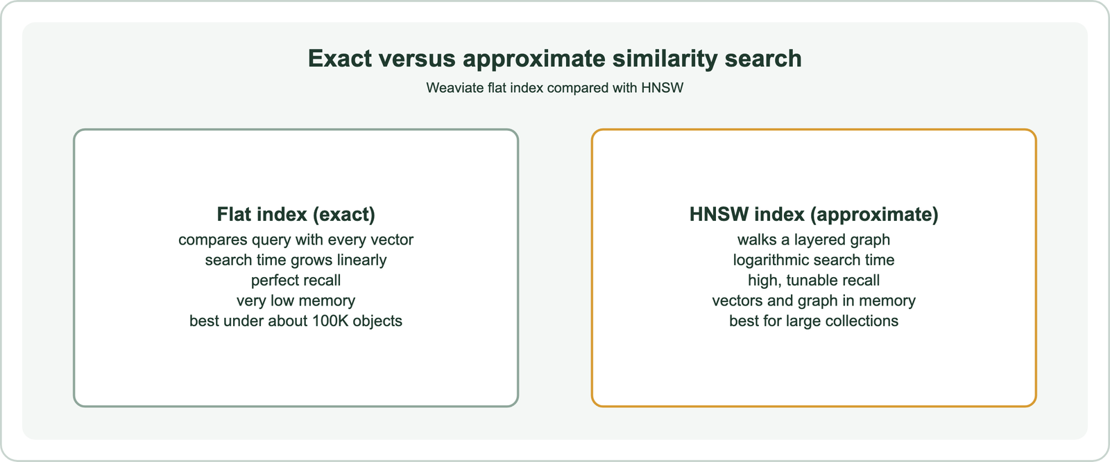
Weaviate Academy gives a simple rule of thumb. Under about 100,000 objects, a flat index offers perfect accuracy with acceptable speed. Above that, HNSW scales to very large collections. A dynamic index starts flat and converts to HNSW at a threshold, 10,000 objects by default, and the switch is one-way.
Other approximate methods exist. Locality-sensitive hashing, introduced for this purpose by Gionis, Indyk, and Motwani in 1999, hashes vectors so similar ones tend to share buckets. Cluster-based indexes search only the most promising groups. FAISS, described by Johnson, Douze, and Jegou in 2017, implements many of these methods for billion-scale search. Approximate nearest neighbor search and exact versus approximate search go deeper. Speed, though, says nothing about whether the results are any good.
Does the nearest result always mean a relevant result?
The nearest result does not always mean a relevant result, because similarity search always returns the closest items, even when nothing in the collection matches well. Every vector is some distance from every other vector.
Weaviate’s documentation states this plainly. All compatible vectors are similar to some degree, so there will always be top results regardless of relevance. Its example is a collection holding only the colors red, crimson, and light coral. A query for sky blue still returns red, because red is the closest match, not because it is a good one.
Weaviate provides four controls to deal with this:
- Limit caps the number of results, with a default of 10 set by
QUERY_DEFAULTS_LIMIT. - Threshold sets a maximum distance, so weak matches are dropped.
- Autocut stops at natural jumps in the distance values.
- Filters exclude results by properties such as date, category, or tenant.
Autocut is the least familiar of the four, and the reference gives a clear example. A query returns distances of 0.1899, 0.1901, 0.191, 0.21, 0.215, and 0.23. The jump after 0.191 marks a natural break. Autocut set to 1 returns the first three results. Set to 2, it returns five, stopping at the next jump.
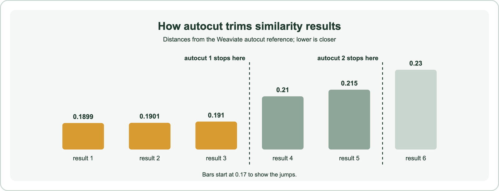
Weaviate’s recommended practice is to combine them: start with a limit, then tune a threshold so irrelevant results are unlikely to appear. Relevance scores and top-k retrieval explain how scores and cut-offs interact. All of these controls are parameters on a single query.
How do you run a similarity search in Weaviate?
You run a similarity search in Weaviate with a near_text, near_vector, or near_object query on a collection, adding a limit, distance threshold, or autocut as needed. The Python v4 client exposes each as a method on collection.query.
import weaviate
from weaviate.classes.query import MetadataQuery, Filter

client = weaviate.connect_to_local()
articles = client.collections.use("Article")

# Text query: Weaviate embeds it with the collection's vectorizer
response = articles.query.near_text(
    query="how to lower cloud costs",
    distance=0.35,          # drop anything farther than this
    limit=10,
    filters=Filter.by_property("language").equal("en"),
    return_metadata=MetadataQuery(distance=True),
)
for obj in response.objects:
    print(round(obj.metadata.distance, 3), obj.properties["title"])

# "More like this": reuse an existing object's vector
similar = articles.query.near_object(near_object=response.objects[0].uuid, limit=5)

client.close()
The distance threshold follows the collection’s metric. With the default cosine metric, distances run from 0 to 2, so a value such as 0.35 keeps only close matches. A good threshold depends on the model and the data, so it should be tuned on real queries rather than copied. Weaviate’s documentation notes that distance and certainty cannot be combined, and that certainty applies only to cosine.
For collections without a vectorizer, near_vector takes a vector computed elsewhere. Its length must match the vectors in the collection. The build guide covers setting up the collection itself. Outside a database, the same idea applies to just two pieces of text.
How can you measure the similarity between two texts?
You can measure the similarity between two texts by embedding both with the same model and computing the cosine similarity of the two vectors, where values closer to 1 mean closer meaning. Lexical measures such as word overlap are a simpler alternative that ignores meaning.
The embedding approach takes a few lines of Python with the Sentence Transformers library. The all-MiniLM-L6-v2 model outputs 384-dimension vectors, and util.cos_sim returns their cosine similarity.
from sentence_transformers import SentenceTransformer, util

model = SentenceTransformer("all-MiniLM-L6-v2")
a, b, c = model.encode([
    "How do I reset my password?",
    "Steps to recover a forgotten login",
    "Best hiking trails near Denver",
])
print(util.cos_sim(a, b))  # related meaning, few shared words
print(util.cos_sim(a, c))  # unrelated topic
The first pair shares almost no words but should score clearly higher than the second, because the model places both near the idea of account recovery. The exact numbers vary by model, so compare scores within one model, not across models.
Lexical methods answer a different question. Jaccard similarity divides the shared words by the total distinct words. It is fast and transparent but scores the password pair near zero. Keyword ranking such as BM25 works the same way at search scale, as BM25 versus vector search explains. Choosing between word overlap and meaning is also the clearest way to see how similarity search relates to semantic search.
What is the difference between similarity search and semantic search?
The difference between similarity search and semantic search is that similarity search is the mechanism, ranking items by vector distance, while semantic search is the goal, returning results that match a query’s meaning. Semantic search usually runs on similarity search, but the two are not the same thing.
Weaviate draws the line the same way. Its explainer notes that the terms vector search, similarity search, and semantic search are often used interchangeably. It adds that semantic search describes the user experience, while vector search describes the technical mechanism.
| Aspect | Similarity search | Semantic search |
|---|---|---|
| What it is | A mechanism: nearest neighbors by distance | A goal: results that match meaning and intent |
| Data | Any vectors: text, images, audio, user behavior | Mostly text and natural language queries |
| Needs meaning? | No; works on any numeric features | Yes; depends on embeddings that capture meaning |
| Extra layers | Index and metric | Query understanding, hybrid search, reranking |
Two consequences follow. Similarity search can work without any notion of meaning, for example on audio fingerprints or product feature vectors. And semantic search can use more than similarity search, such as keyword matching in hybrid search or a second-stage reranker. The overview of what semantic search is covers the full picture. That broader reach shows up in where similarity search is used.
Where is similarity search used?
Similarity search is used wherever a system must find items like a given one, including semantic text search, recommendations, image and audio lookup, duplicate detection, and retrieval for RAG. The mechanism stays the same; only the embeddings change.
- Semantic search: documents are ranked by closeness in meaning to the query, as in these semantic search examples.
- Retrieval for RAG: the passages nearest a question are passed to a language model as context.
- Recommendations: items near what a user viewed or liked are suggested, often through a “more like this” query.
- Image and video search: Weaviate’s
nearImageandnearVideoqueries find visually or conceptually similar media. - Music and audio: audio embeddings let a system find songs or sounds that resemble a sample.
- Duplicate and fraud detection: near-identical records, listings, or transactions sit close together.
- Multilingual search: models that map languages into one space find matches across languages.
Weaviate’s documentation sums up when the approach fits: vector search is best suited where a human-like idea of similarity is a good measure of result quality. The semantic search use cases page goes further on text applications. Where that idea of similarity breaks down, the limits show.
What are the limits of similarity search?
The limits of similarity search are that it finds closeness rather than correctness, depends entirely on the embedding model, misses exact terms, and costs memory and compute at scale. Each limit has a known mitigation.
- Closeness is not relevance: the nearest item may still be wrong. Thresholds, autocut, and reranking help.
- Model dependence: results are only as good as the embeddings. A model trained on general text may miss domain terms, which is why teams test models and sometimes fine-tune them.
- Exact terms: product codes, names, and rare words can be blurred by embeddings. Hybrid search adds keyword matching back.
- Approximation: ANN indexes can miss true neighbors. Recall should be measured, as in recall at k.
- Cost: vectors and graph indexes use memory, and distance math uses CPU. Compression and smaller embedding dimensions reduce both.
- Hard to explain: a distance score does not say why two items are close, which matters in regulated settings.
None of these limits removes the value of the method. They mean similarity search works best as one stage in a system, combined with filters, keyword signals, and evaluation. Metadata filtering, vector indexes, vector search, dense vectors, and semantic matching cover the neighboring pieces.
Similarity search finds the items closest to a query by embedding both and measuring vector distance with a metric such as cosine. Small collections can use exact, brute-force comparison, while large ones use approximate indexes such as HNSW and accept a tunable loss in recall. Because every vector is near something, limits, thresholds, autocut, and filters keep weak matches out. Similarity search is the mechanism; semantic search is the goal it serves, alongside keyword matching and reranking. The practical step is to choose the metric your model was trained with, test a threshold on real queries, and measure recall.