Home / Scale and cost / GPU-Accelerated Vector Search: When It Is Worth It

GPU-Accelerated Vector Search: When It Is Worth It

GPU-accelerated vector search uses graphics processors to build vector indexes and answer nearest neighbour queries, exploiting thousands of parallel cores to compute many distances at once. It is worth it when index builds are large or frequent, or when query volume is high enough to fill the GPU with batched work. It rarely pays off for small collections or light traffic, where CPU indexes such as HNSW are already fast and much cheaper. The main GPU index today is CAGRA, a graph index designed for GPUs and available in NVIDIA’s cuVS library. Weaviate’s early benchmarks with cuVS reported index builds 4.7 times faster than CPU HNSW at 1 million vectors and 5.4 times faster at 8.7 million, with end-to-end queries 2.6 and 3.5 times faster. A practical middle path builds the index on a GPU and serves it on CPUs. GPU memory limits how much data fits, so compression and sizing come first.

What is GPU-accelerated vector search?

GPU-accelerated vector search is vector search in which the heavy numeric work, building the index and computing distances between vectors, runs on a graphics processor instead of a CPU. The results are the same kind of nearest neighbours; only the hardware changes.

Vector search finds stored vectors closest to a query vector. Exact search compares the query with every vector. Approximate indexes such as HNSW reduce the comparisons by walking a graph, as described in scaling semantic search. Either way, most of the time goes into distance calculations: thousands of multiply-and-add operations per comparison.

That kind of arithmetic suits GPUs. A GPU has thousands of simple cores built to run the same operation on many numbers at once, which is why GPUs also train neural networks. Libraries for GPU vector search include FAISS, whose GPU implementation was described by Jeff Johnson, Matthijs Douze and Hervé Jégou in 2017, and NVIDIA’s cuVS.

The GPU can help at two points. Index building runs once per dataset or model change and is very heavy. Query serving runs continuously and is lighter per request but constant. The gains differ at each point, and so does the cost case. The reasons start with how GPUs process work.

Why are GPUs fast at vector search?

GPUs are fast at vector search because distance calculations are highly parallel, and a GPU can compute thousands of them at the same time with very high memory bandwidth. The speed only appears when there is enough work to fill the device.

A single comparison between two 768-dimension vectors is 768 multiplications and additions. A query against a million candidates, or a batch of queries against a graph neighbourhood, is millions of such operations that do not depend on each other. A CPU core works through them a few at a time. A GPU spreads them across its cores.

Batching is what makes this pay. A single query walking a graph index takes a sequence of small steps, and each step depends on the last. On its own it cannot fill a GPU. Many queries processed together can. Weaviate’s blog on its NVIDIA integration notes that Weaviate batches incoming queries to exploit the GPU’s parallelism, particularly during peak loads, without manual batching from the user.

Moving data also costs time. Vectors must travel from host memory to GPU memory, and results must come back. Weaviate’s blog describes contributions to cuVS for pooled memory, which pre-allocates GPU memory for small allocations, and pinned memory, which keeps host memory from being paged out so transfers are faster. Graph indexes also had to be redesigned for GPUs.

How does the CAGRA index differ from HNSW?

CAGRA is a graph-based approximate nearest neighbour index built for GPUs, with a fixed-degree graph and a search procedure designed for massive parallelism. HNSW was designed for CPUs and uses a layered graph.

CAGRA was introduced by Hiroyuki Ootomo and colleagues at NVIDIA in 2023. Weaviate’s blog describes it as a GPU-native vector search algorithm designed from the ground up for the parallel processing capabilities of GPUs. It is part of cuVS, NVIDIA’s open-source library of vector search algorithms, which also includes IVF-based indexes.

HNSW, the default vector index in Weaviate, builds a hierarchy of graph layers and searches greedily from the top layer down. Its structure suits a CPU walking one path per query. CAGRA uses a single-layer graph in which every node has the same number of neighbours, a regular shape that lets a GPU explore many candidates per step and handle many queries side by side.

The two graphs are related closely enough to convert. Weaviate’s blog describes a cuVS feature that converts a CAGRA-built index into an HNSW index. That conversion is the basis of a hybrid deployment pattern. The reported speed-ups explain why it matters.

What speed-ups has Weaviate reported for GPU vector search?

Weaviate reported index builds 4.7 to 5.4 times faster and end-to-end queries 2.6 to 3.5 times faster with NVIDIA cuVS than with HNSW on a 16-core CPU. The early benchmarks used 1 million and 8.7 million vectors. The gains grew with dataset size.

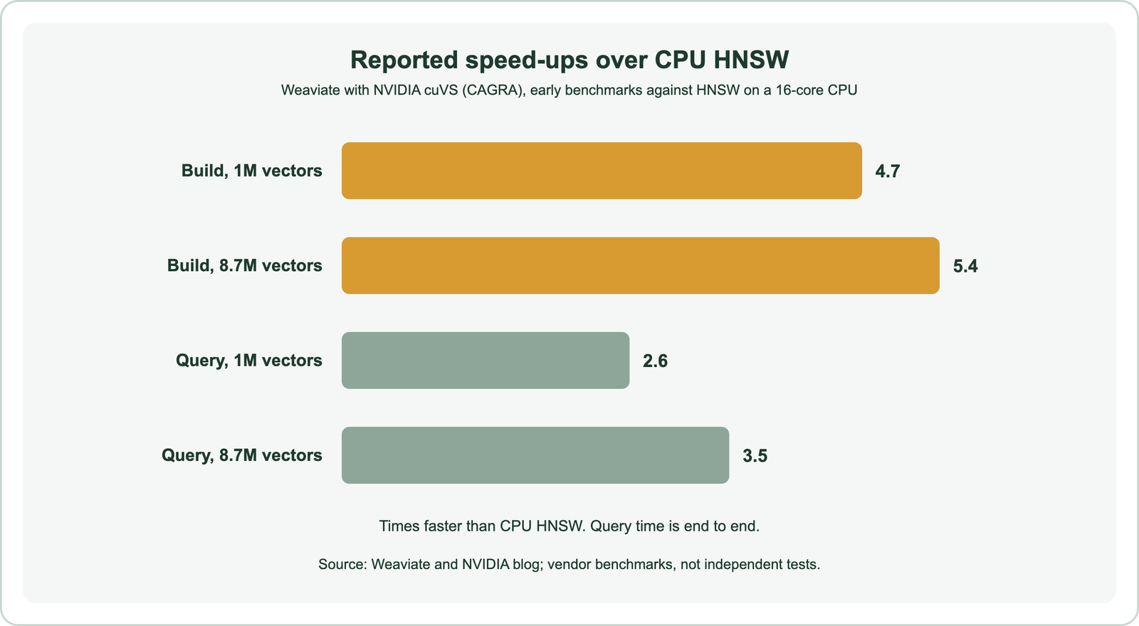
The figures come from Weaviate’s blog on its work with NVIDIA, presented first at NVIDIA’s GTC conference. At 1 million vectors, index builds were 4.7 times faster and end-to-end queries 2.6 times faster. At 8.7 million vectors, builds were 5.4 times faster and queries 3.5 times faster. The blog also reports more than a further threefold improvement on the NVIDIA DGX B200 platform.

Read these as indications, not guarantees. They compare particular GPUs with a particular 16-core CPU, on particular datasets and settings. Speed-ups depend on dimensions, recall targets, batch sizes and hardware generations. The blog does not present them as independent tests.

The pattern is still informative. Builds gained more than queries, and both gained more at the larger size. That fits the earlier reasoning: index building is the most parallel work, and larger datasets give the GPU more to do. It also points to the deployment pattern that captures the build gain cheaply.

Can a GPU-built vector index be served on CPUs?

A GPU-built vector index can be served on CPUs by building a CAGRA graph with cuVS and converting the graph to an HNSW index, which then runs on ordinary CPUs. Weaviate’s blog describes this as a hybrid GPU-build, CPU-serve architecture.

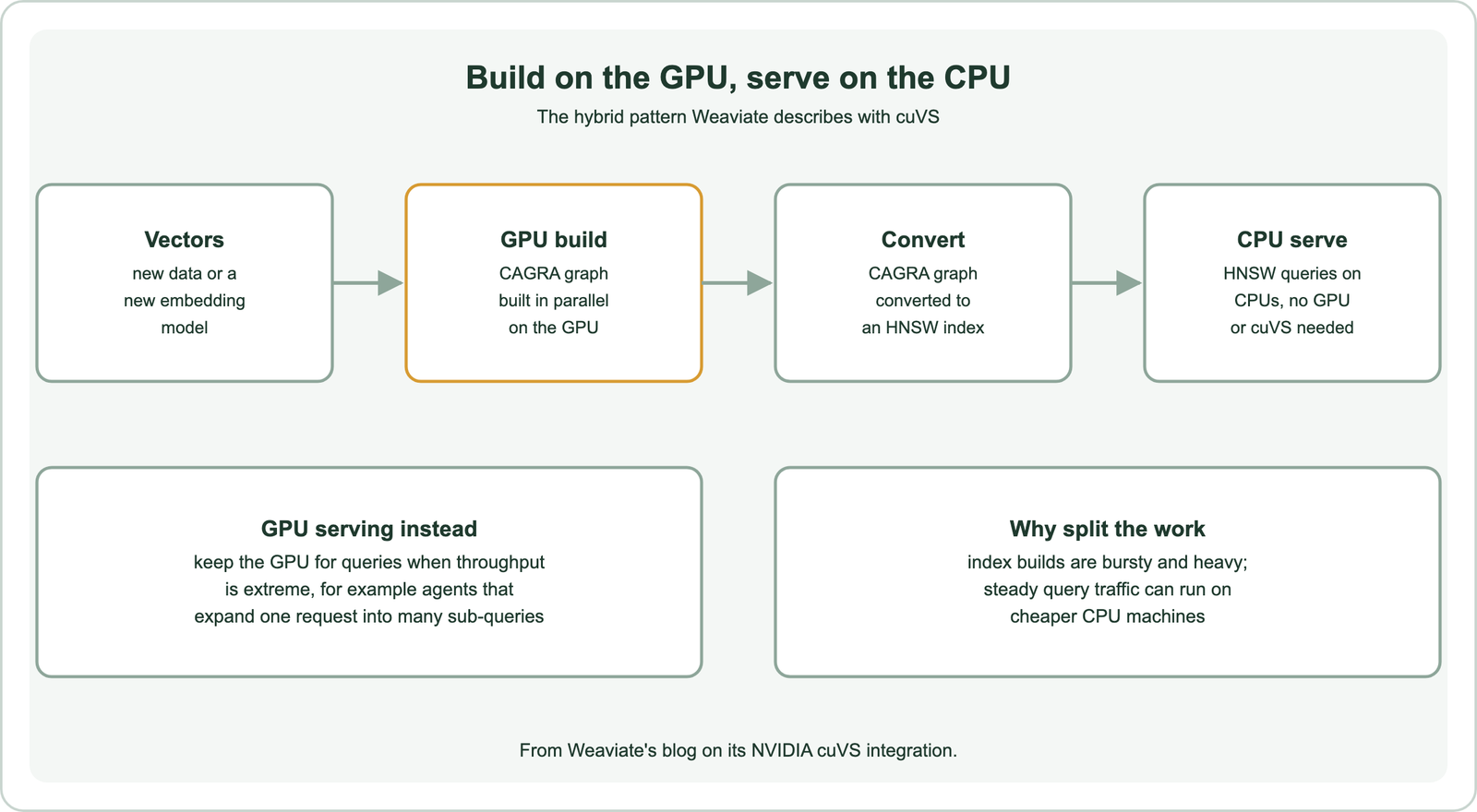
According to the blog, after conversion the served HNSW index has no dependency on GPUs or cuVS. The GPU is needed only while building. Teams can rent GPU time for a rebuild, then serve queries on the CPU machines they already run.

This suits the way index work arrives. Rebuilds happen in bursts: a new embedding model, a large data load or a schema change. Weaviate’s blog notes that billion-object datasets can take hours or even days to build on CPUs, and that long re-indexing times slow down adoption of better embedding models. A faster build shortens that loop, a concern covered in real-time indexing and index freshness.

Serving on GPUs remains an option when query volume is extreme. The blog points to agents as a source of such volume, since query rewriting can expand one request into dozens or hundreds of sub-queries. Whether either pattern is worth it depends on the workload.

When does GPU vector search pay off?

GPU vector search pays off when you rebuild large indexes often, when query volume is high enough to batch, or when re-embedding with new models is slowed by index build time. It rarely pays off for small or quiet workloads.

Frequent large rebuilds are the clearest case. If a collection of tens of millions of vectors must be re-indexed for each new embedding model, build time decides how fast you can move. The cost side is covered in the cost of semantic search.

High query volume is the second case. Agentic systems multiply searches. In an illustrative case, 20 user requests per second that each expand into 50 sub-queries make 1,000 searches per second. Loads like that keep a GPU busy with batched work. Fewer, steadier queries may never fill one.

Small collections are the counter case. A few hundred thousand vectors fit in CPU memory and HNSW answers in milliseconds. The GPU’s transfer overhead and cost add little. Weaviate’s default CPU HNSW index handles most applications, and the trade-off between recall and speed on it is explained in the recall vs latency trade-off. Memory is the constraint that decides how much fits.

How much GPU memory does vector search need?

Vector search needs GPU memory for the vectors and the index, roughly the number of vectors times dimensions times bytes per value, plus graph overhead. Raw float32 vectors use 4 bytes per value.

def vector_memory_gb(n_vectors, dims, bytes_per_value=4):
    return n_vectors * dims * bytes_per_value / 1e9

print(vector_memory_gb(10_000_000, 768))      # 30.72  (float32)
print(vector_memory_gb(10_000_000, 768, 1))   # 7.68   (8-bit values)
print(vector_memory_gb(100_000_000, 768))     # 307.2  (float32)

Ten million 768-dimension vectors take 10,000,000 × 768 × 4 bytes, which is 30.72 GB, before any graph edges. Storing each value in one byte brings that to 7.68 GB. One hundred million float32 vectors need 307.2 GB, more than a single GPU typically holds, so such datasets must be compressed, split across devices or built in parts.

The same arithmetic applies to CPU memory, which is usually larger and cheaper per gigabyte. That is one more reason the build-on-GPU, serve-on-CPU pattern appeals. Compression trades a little recall for space, as with the quantization options covered in scaling semantic search. Memory is one of several limits.

What are the drawbacks of GPU vector search?

The drawbacks of GPU vector search are cost, limited device memory, the need for batching to reach full speed, data transfer overhead and extra operational complexity. Each can erase the speed gain for the wrong workload.

Cost comes first. GPU machines cost more per hour than CPU machines, so the speed-up must exceed the price difference to save money, unless faster builds have value of their own. Batching trades latency for throughput: waiting to group queries adds delay to each one, which matters for interactive search, as discussed in search latency.

Operations get harder. GPU drivers, library versions and device scheduling add moving parts. Features such as filtering, hybrid keyword search and multi-tenancy must work on the GPU path too, or queries fall back to the CPU. Managed services can hide this work, a choice weighed in managed vs self-hosted search.

Measure before buying. Benchmark your own data, dimensions, recall target and traffic shape on CPU HNSW first. Then test a GPU build and, separately, GPU serving. Count total cost per rebuild and per million queries, not only speed.

GPU-accelerated vector search runs index builds and distance calculations on graphics processors, using parallelism and batching. CAGRA, in NVIDIA’s cuVS library, is the main GPU graph index. Weaviate’s early benchmarks reported builds 4.7 to 5.4 times faster and queries 2.6 to 3.5 times faster than HNSW on a 16-core CPU. A CAGRA index can be converted to HNSW, so a GPU can build and CPUs can serve. GPUs pay off for large, frequent rebuilds and very high query volume, including agentic query expansion. For small collections and light traffic, CPU HNSW remains cheaper. Size memory first: 10 million 768-dimension float32 vectors need 30.72 GB.