Home / Search evaluation / nDCG Explained: Normalized Discounted Cumulative Gain

nDCG Explained: Normalized Discounted Cumulative Gain

nDCG, or normalized discounted cumulative gain, is a ranking metric that sums the position-discounted relevance grades of a result list. It then divides that sum by the best score possible for the query. It answers two questions at once: did the system find the most relevant documents, and did it put them at the top? Graded relevance is its distinctive feature. A highly relevant document counts more than a somewhat relevant one, which precision, recall and MRR cannot express. The discount, usually one over the base-2 logarithm of the rank plus one, makes rank 1 count fully and later ranks progressively less. Dividing by the ideal ordering puts every query on a 0 to 1 scale, so scores can be averaged. nDCG at 10 is the standard headline metric for retrieval benchmarks, including the MTEB leaderboard’s retrieval category.

What is nDCG in search evaluation?

nDCG in search evaluation is a score between 0 and 1 that measures how close a ranked result list comes to the best possible ordering, given graded relevance judgments. A score of 1 means the system ranked the judged documents in the ideal order.

Kalervo Järvelin and Jaana Kekäläinen introduced cumulative gain measures in their 2002 paper “Cumulated gain-based evaluation of IR techniques”. Their goal was to reward systems for putting highly relevant documents first, which binary metrics could not do. A ranking that buries the best answer at rank 8 behind somewhat relevant ones should score worse than one that leads with it.

A Weaviate blog post on evaluation metrics groups nDCG with MAP and MRR as rank-aware metrics, as opposed to precision and recall, which only count relevant items. It also notes that nDCG requires knowing not just whether a document is relevant but how relevant it is. That requirement is both the metric’s strength and its cost, because graded judgments take more effort to collect.

The name lists the three steps in reverse. Gain is the relevance grade. Cumulative means adding gains down the list. Discounted means reducing the gain at lower ranks. Normalized means dividing by the ideal. Each step deserves a look, starting with gain. The metric family is surveyed in information retrieval metrics.

What does cumulative gain measure?

Cumulative gain measures the total relevance of the top k results by adding up each result’s relevance grade, without regard to order. It rewards finding relevant documents and rewards highly relevant ones more.

Relevance grades come from judgments. A common scale runs from 0 for not relevant to 3 for highly relevant. If the top four results have grades 3, 1, 0 and 2, their cumulative gain is 6. A list with grades 0, 0, 1, 1 has a cumulative gain of 2. The first list is better, and the number says so.

Cumulative gain alone ignores position. The list 0, 2, 1, 3 also sums to 6, even though its best document sits at rank 4. Users read from the top and often stop early, so a metric that ignores order misjudges what they experience. That is why the discount exists.

Grades also need a consistent scale. Weaviate’s academy course on evaluation stresses grading every document on one scale and using that scale everywhere, because mixing scales silently produces wrong scores rather than errors. Building such judgments is covered in search test sets and relevance judgments. The discount turns this sum into a ranking metric.

How does the discount in nDCG work?

The discount in nDCG works by dividing the gain at rank i by the base-2 logarithm of i plus one, so rank 1 keeps its full gain and later ranks keep less. The sum of discounted gains is DCG.

The discount values follow from the formula. Rank 1 divides by log2(2), which is 1. Rank 2 divides by log2(3), about 1.585, keeping about 0.631 of the gain. Rank 3 divides by log2(4), which is 2, keeping 0.5. Rank 4 divides by log2(5), about 2.322, keeping about 0.431. Weaviate’s evaluation article gives the same formula: DCG at K is the sum of each relevance grade divided by log2(i + 1).

The logarithm decays slowly. Rank 10 still keeps about 0.289 of its gain, so documents deep in a list still count. That suits ranked result pages, where users scan several results. Metrics such as MRR, which stops at the first relevant result, model a user who wants one answer, as covered in mean reciprocal rank.

DCG on its own cannot be compared across queries. A query with ten highly relevant documents can reach a much higher DCG than a query with one. A score of 4.5 might be excellent for one query and poor for another. Normalization solves that.

How does normalization turn DCG into nDCG?

Normalization turns DCG into nDCG by dividing it by the ideal DCG, the DCG of the best possible ordering of all judged documents for that query. The result lies between 0 and 1 for every query.

The ideal ordering sorts every judged document by grade, highest first, and keeps the top k. Its DCG, called IDCG, is the most any system could score on that query. nDCG at k is DCG at k divided by IDCG at k, the definition given in Weaviate’s evaluation article.

The ideal must come from all judged documents, not only the ones the system returned. A relevant document the system missed belongs in the ideal list, and leaving it out inflates the score. Standard tools such as trec_eval build the ideal from the full judgment file. Libraries that compute nDCG from the returned list alone only see what was retrieved.

Once every query is on the same scale, scores can be averaged into one number for the whole test set. A query with no relevant judged documents has an IDCG of zero, so its nDCG is undefined; tools differ in whether they skip it or score it as zero, so check the convention. A worked example makes the steps concrete.

How do you calculate nDCG step by step?

You calculate nDCG step by step by listing the grades of the top k results, discounting each by its rank, summing to DCG, doing the same for the ideal order, and dividing. The example uses k = 4 and linear gain.

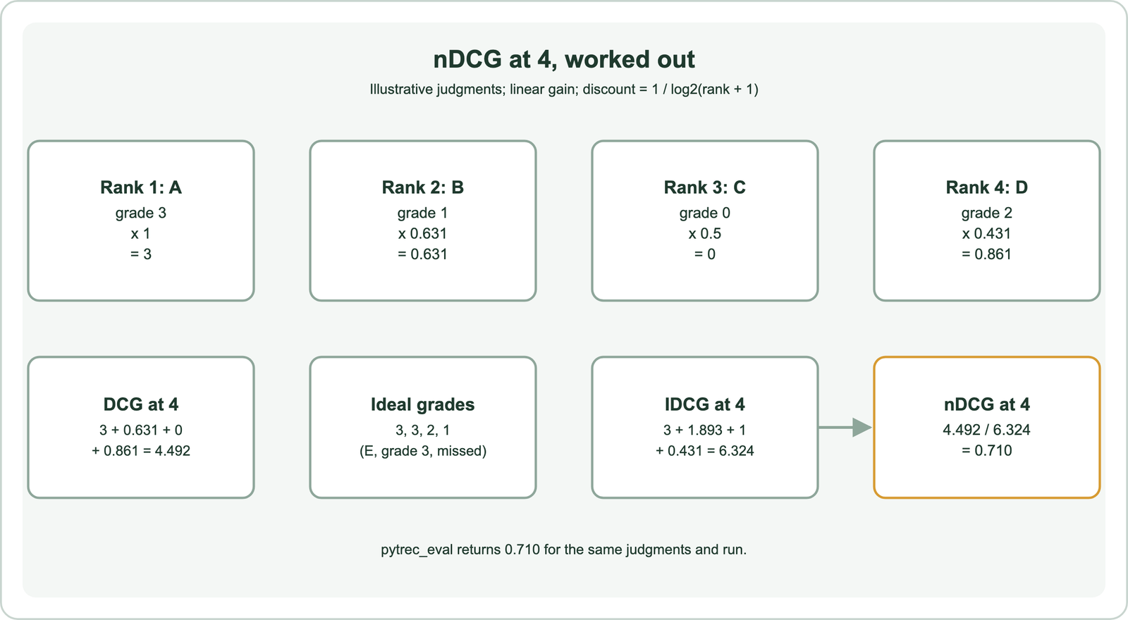
A query has five judged documents. A has grade 3, B grade 1, C grade 0, D grade 2 and E grade 3. The system returns A, B, C, D, and never finds E. The discounted gains are 3 × 1, 1 × 0.631, 0 × 0.5 and 2 × 0.431. Their sum, the DCG at 4, is about 4.492.

The ideal top four takes the highest grades from all judgments: 3, 3, 2, 1. Its discounted gains are 3, 1.893, 1 and 0.431, summing to an IDCG of about 6.324. nDCG at 4 is 4.492 divided by 6.324, which is about 0.710. The pytrec_eval library, which wraps trec_eval, returns the same 0.710 for these judgments.

Two changes would raise the score. Moving D above B swaps a grade 1 at rank 2 for a grade 2. Finding E and placing it second adds a grade 3 near the top. The metric rewards both, which is what a ranking metric should do. The same arithmetic changes, though, if the gain is defined differently.

How do linear and exponential gain change nDCG?

Linear and exponential gain change nDCG by weighting high grades differently: linear gain uses the grade itself, while exponential gain uses 2 to the power of the grade, minus 1. Exponential gain makes the top grade count far more than the next one.

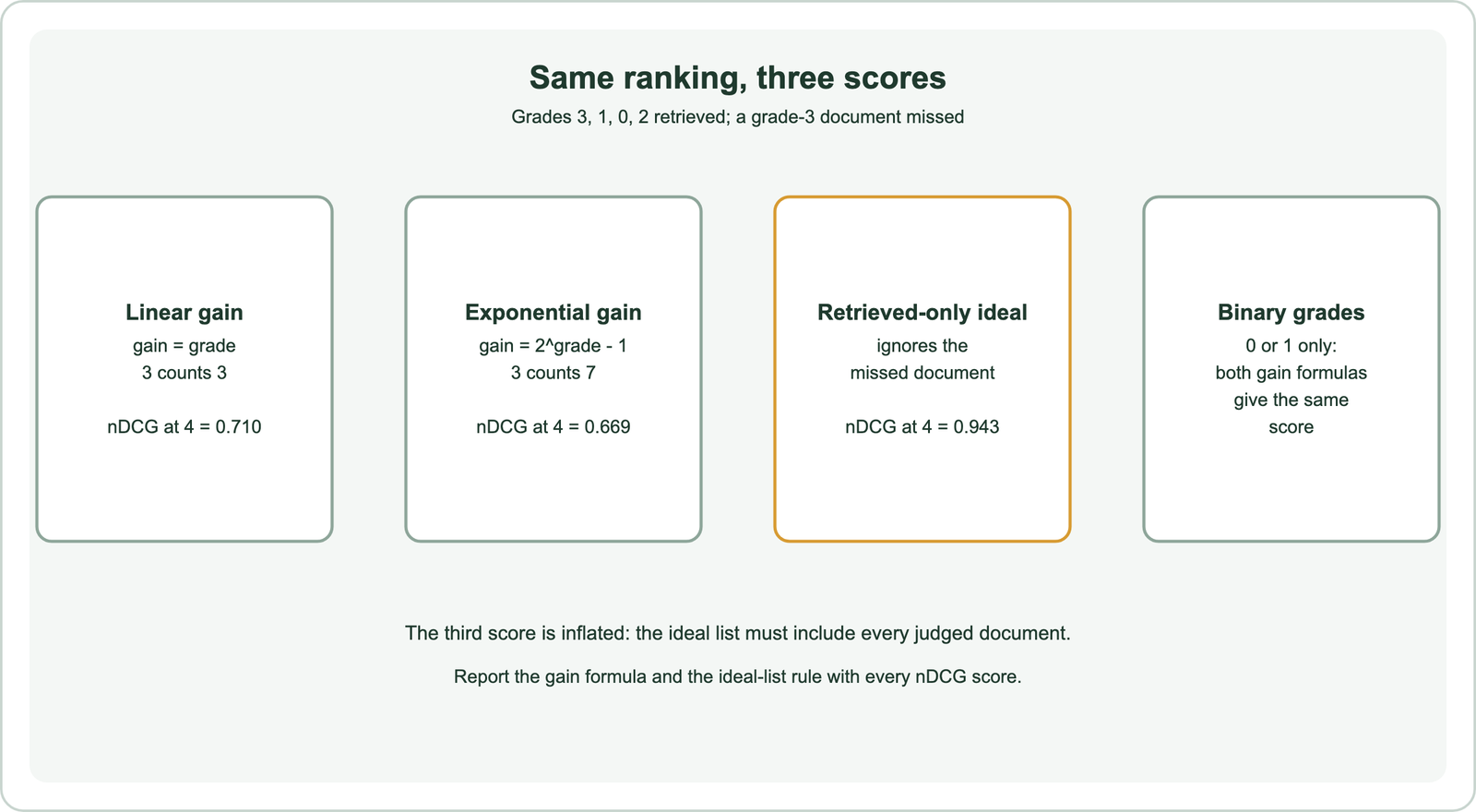
Weaviate’s evaluation article uses linear gain in its DCG formula. Weaviate’s academy course uses exponential gain, 2 to the power of the score minus 1, and notes that a grade of 3 then contributes 7 while a grade of 2 contributes 3. The exponential form was popularized by learning-to-rank work such as Burges and colleagues’ RankNet paper in 2005.

For the worked example, exponential gain gives a DCG of about 8.923 and an IDCG of about 13.347, so nDCG at 4 falls to about 0.669. The missed grade-3 document now costs more, because grade 3 is worth 7 rather than 3. Neither variant is wrong. They encode different views of how much better a perfect result is than a good one.

With binary grades of 0 and 1, the two forms agree, because 2 to the power of 1, minus 1, is 1. The difference appears only with graded judgments. Always state the variant next to a reported score, or comparisons across papers and tools mislead. The tooling choice raises a second trap.

How do you compute nDCG in Python?

You compute nDCG in Python with pytrec_eval, passing the full relevance judgments and the system’s scored results, so the ideal list includes documents the system missed. It reproduces trec_eval, the standard tool from the TREC evaluations.

import pytrec_eval

qrels = {"q1": {"A": 3, "B": 1, "C": 0, "D": 2, "E": 3}}   # all judged documents
run = {"q1": {"A": 4.0, "B": 3.0, "C": 2.0, "D": 1.0}}     # system scores, higher first

evaluator = pytrec_eval.RelevanceEvaluator(qrels, {"ndcg_cut.4", "ndcg_cut.10"})
print(evaluator.evaluate(run)["q1"]["ndcg_cut_4"])         # 0.7104...

The qrels dictionary holds every judgment, including E, which the system never returned. The run dictionary holds the system’s scores, which pytrec_eval sorts to get the ranking. The ndcg_cut measures compute nDCG at each cut-off with linear gain.

A common mistake is passing only the retrieved documents’ grades to a function that builds the ideal from its input. scikit-learn’s ndcg_score, called with the grades 3, 1, 0, 2 and the system’s scores, returns about 0.943 for the same example, because it never sees E. That score describes ordering among retrieved documents, not retrieval quality. For search evaluation, include unretrieved judged documents in the ideal.

The judgments themselves must exist before any of this. Weaviate’s academy course notes that even 20 objects with multiple queries can yield meaningful results for a custom benchmark. A complete workflow is in how to evaluate semantic search. Choosing the cut-off is the next decision.

How should you choose k and read nDCG scores?

You should choose k to match how many results users or a language model actually consume, and read nDCG scores only relative to other systems on the same judgments. nDCG at 10 is the benchmark convention, not a rule for every product.

A search page that shows ten results fits nDCG at 10. A RAG pipeline that passes five passages to a model fits nDCG at 5, or recall at 5, since the model reads all five regardless of order. A question-answering box that shows one answer fits MRR or success at 1. The related counting metrics are covered in recall at k and precision at k.

Absolute values do not transfer between datasets. An nDCG at 10 of 0.5 can be strong on a hard benchmark and weak on an easy one, because it depends on the queries, the corpus and the judging. Public leaderboards built on BEIR and MTEB compare models on fixed judgments, as covered in retrieval benchmarks. Your own test set is what predicts your own results.

nDCG can also miss problems. Incomplete judgments treat unjudged documents as irrelevant, which penalizes systems that find good documents nobody judged. Averages hide queries that fail entirely. Inspect the worst queries, not just the mean. The difference between relevance and coverage is explored in relevance vs recall, and failure patterns in why vector search returns irrelevant results.

When should you use nDCG instead of other search metrics?

You should use nDCG when relevance has degrees and the order of results matters, as on ranked result pages and in comparisons of embedding models or rerankers. Other metrics fit other questions better.

Weaviate’s academy course describes nDCG as often ideal for retrieval benchmarks because it rewards systems for prioritizing highly relevant results. Weaviate’s evaluation article notes that nDCG is highly popular for retrieval systems, while MAP is more common for recommendation systems. It is the natural choice when comparing two embedding models or tuning a hybrid alpha on graded judgments.

Some questions need different tools. ANN recall measures whether an approximate index returns the true nearest neighbours, which is an engineering check rather than a relevance one, as covered in ANN recall. Online metrics such as click-through and abandonment measure what real users do, as described in online search metrics and analytics.

In production, offline nDCG and online signals complement each other. A change that raises nDCG on the test set should also hold up with users. Ongoing tracking is covered in monitoring search quality in production.

nDCG scores a ranked list by summing graded relevance, discounting each grade by one over log2 of rank plus one, and dividing by the ideal ordering of all judged documents. In the worked example, a list with grades 3, 1, 0, 2 and a missed grade-3 document scores 0.710 with linear gain and 0.669 with exponential gain. Build the ideal from every judgment, state the gain variant, choose k to match what users or the model consume, and compare scores only on the same judgments. Use nDCG when relevance has degrees and order matters.