Home / Foundations / The Curse of Dimensionality in Vector Search

The Curse of Dimensionality in Vector Search

The curse of dimensionality is the set of problems that appear when data has many dimensions. Space grows so fast that points become sparse, distances between them grow similar, and exact search structures stop working well. Embeddings used in semantic search often have hundreds or thousands of dimensions, so the effect matters in practice. For random points, the gap between the nearest and the farthest neighbour shrinks as dimensions grow, which threatens the idea of a “nearest” neighbour. Real embeddings escape the worst of it because they are not random: related items cluster on structures with far fewer effective dimensions. Search systems still pay a price. Exact indexes such as k-d trees degrade towards brute force, so vector databases use approximate nearest neighbour indexes such as HNSW, which Weaviate uses by default, along with compression to keep large vectors affordable.

What is the curse of dimensionality?

The curse of dimensionality is the observation that many methods that work well in two or three dimensions become inefficient or unreliable as the number of dimensions grows. The term covers several related effects rather than one law.

The first effect is sparsity. The volume of a space grows exponentially with its dimensions, so a fixed number of points spreads ever thinner. Covering a line with points 0.1 apart takes 10 points; covering a square at the same spacing takes 100; a cube takes 1,000; and 10 dimensions take 10,000,000,000. No realistic dataset fills a high-dimensional space.

The second effect is distance concentration. For many kinds of random data, the distances from a query to its nearest and farthest neighbours become nearly equal as dimensions grow. If every point is about equally far away, ranking by distance carries little information.

The third effect is computational. Index structures that split space into regions, such as k-d trees, need to check more and more regions as dimensions grow, until they examine almost every point. These effects all bear on semantic search, which ranks documents by distances between vectors in a high-dimensional vector space.

Where does the term curse of dimensionality come from?

The term curse of dimensionality was coined by the mathematician Richard Bellman in his work on dynamic programming in the late 1950s. He used it for the explosive growth in computation as problems gained more variables.

Bellman’s concern was optimisation: a grid over several variables needs a number of cells that multiplies with each new variable, so exhaustive methods soon become impossible. The same arithmetic applies to sampling, function approximation and search, which is why the phrase spread across statistics, machine learning and databases.

In information retrieval, the term became central once documents were represented as vectors. The vector space model already used one dimension per vocabulary term, which gave sparse vectors with tens of thousands of dimensions. Dense embeddings reduced that to hundreds or thousands, but the geometry of high dimensions still shapes how they behave.

How does space behave in high dimensions?

In high dimensions, almost all the volume of a cube lies in its corners and almost all the volume of a ball lies in a thin shell near its surface. Intuition from two and three dimensions fails.

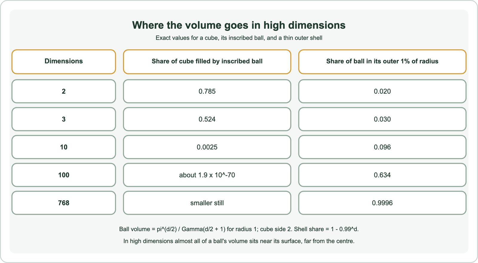
Start with a ball inside a cube that it just touches. In two dimensions, the circle fills about 78.5% of the square. In three, the sphere fills about 52.4% of the cube. In 10 dimensions, the ball fills about 0.25%, and in 100 dimensions the share is about 1.9 × 10^-70. Almost all the cube’s volume is in its corners, far from the centre.

The shell effect is just as striking. The share of a ball’s volume in its outer 1% of radius is 1 − 0.99^d. That is about 2% in two dimensions, about 63% in 100 dimensions and more than 99.9% in 768 dimensions. A random point in a high-dimensional ball is almost certainly near the surface.

These facts explain why sampling and space-partitioning methods struggle. A query’s neighbourhood holds a vanishing share of the space, so finding points near it by dividing space into regions becomes hopeless without additional structure in the data.

Why do distances concentrate in high dimensions?

Distances concentrate in high dimensions because each distance sums contributions from many independent coordinates, and such sums cluster tightly around their average. The relative gap between near and far points shrinks.

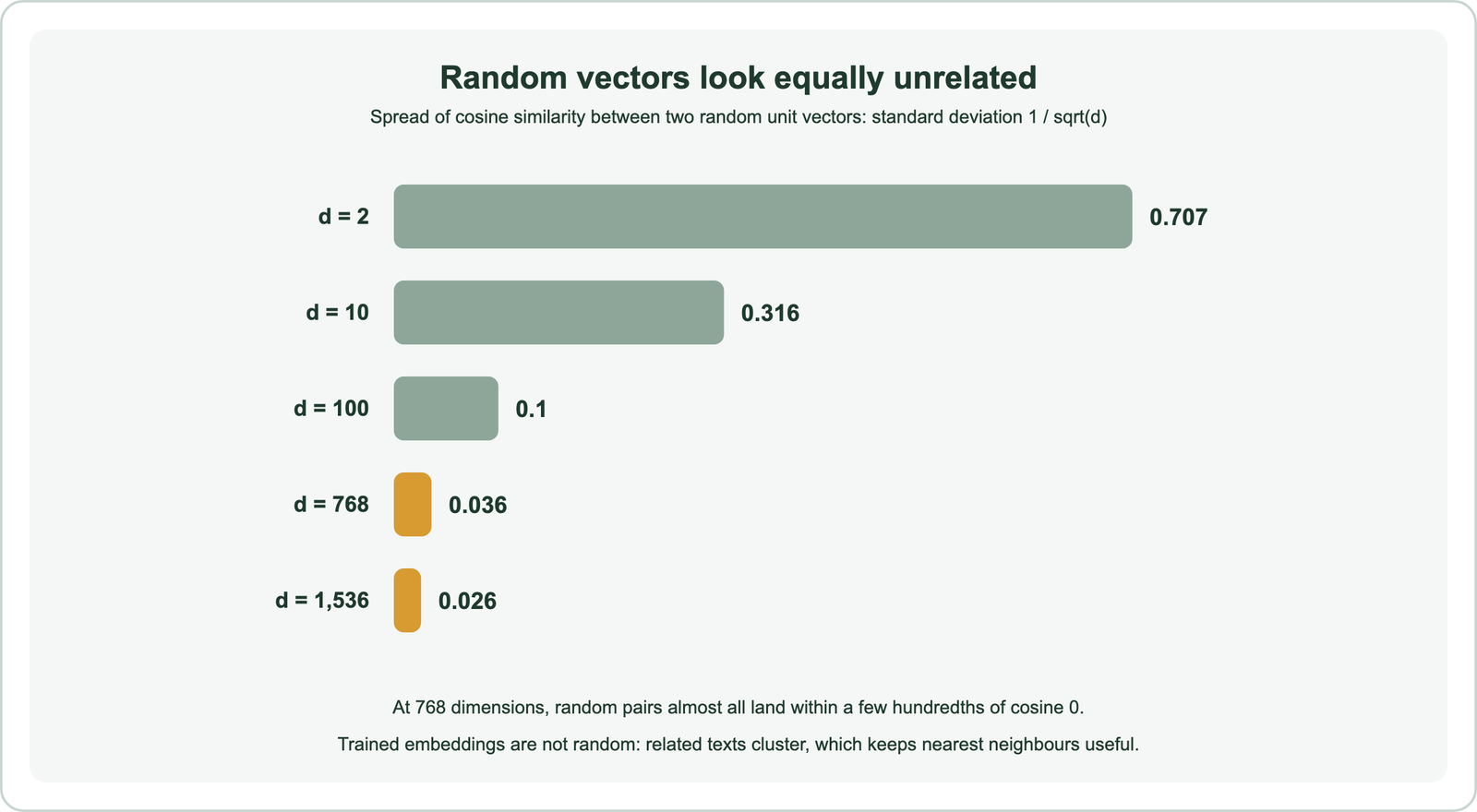
Cosine similarity shows this simply. For two random unit vectors in d dimensions, the cosine has a mean of 0 and a variance of exactly 1/d. In two dimensions the standard deviation is about 0.71, so random pairs take all sorts of angles. In 768 dimensions it is about 0.036, so nearly every random pair sits close to cosine 0, almost exactly at right angles.

Beyer, Goldstein, Ramakrishnan and Shaft formalised the wider effect in a 1999 paper asking when nearest neighbour queries are meaningful. They showed that under broad conditions on the data distribution, the ratio between the farthest and nearest neighbour distances approaches 1 as dimensions grow. The comparison of distance measures in cosine vs dot product vs Euclidean distance is affected in the same way.

The key word is random. The theorem describes data whose dimensions are independent and similarly distributed. Embeddings from trained models do not look like that, which is why semantic search still works.

Does the curse make nearest neighbour search meaningless?

The curse does not make nearest neighbour search meaningless for embeddings, because trained embeddings concentrate on structures with far fewer effective dimensions than their nominal size. Related items sit measurably closer than unrelated ones.

An embedding model is trained to put similar texts close together and different texts far apart. That training creates clusters and directions that carry meaning, so the data occupies a small part of the full space. Its intrinsic dimensionality, the number of directions along which it really varies, is much lower than 768 or 1,536. Distance concentration theorems apply to the full space, not to such structured data.

Beyer and colleagues made this point themselves: nearest neighbour queries stay meaningful when data forms clusters and the query belongs to one. That is the normal case in semantic search, where a query about a topic sits near documents about that topic. Models trained with many dimensions also tend to have redundancy, which techniques such as Matryoshka embeddings exploit by putting the most information in the first dimensions.

The curse still leaves traces. Similarity scores from a given model often fall in a narrow band, so a score of 0.8 from one model can mean something different from 0.8 from another. Ranking by score is reliable; reading absolute scores as probabilities is not. The difference between closeness in meaning and loose association is discussed in semantic similarity vs relatedness.

Why does high dimensionality make exact search slow?

High dimensionality makes exact search slow because space-partitioning indexes lose their pruning power and fall back towards comparing the query with every vector. Each comparison also costs more as vectors get longer.

A k-d tree splits space along one dimension at a time. In low dimensions, a search can skip most branches because they lie far from the query. In high dimensions, the query’s neighbourhood touches almost every branch, as the volume arithmetic suggests, so the tree visits most of them and gains little over a full scan.

A full scan is expensive at scale. Weaviate’s article on vector search gives the arithmetic: comparing a 300-dimensional query with 10 million vectors takes 300 × 10,000,000 = 3 billion operations. The cost grows linearly with both the number of vectors and their dimensions. Exact search remains useful for small collections or heavily filtered subsets, as described in exact vs approximate search.

How do vector search systems cope with high dimensions?

Vector search systems cope with high dimensions by using approximate nearest neighbour indexes, compressing vectors, and trading a small amount of recall for large gains in speed and memory. These methods rely on the structure that real embeddings have.

Graph indexes are the main tool. HNSW, the default index in Weaviate, links each vector to a few of its neighbours and searches by walking the graph towards the query. It does not partition space, so it avoids the corner and shell problems that break trees. The method is explained in approximate nearest neighbour search.

Compression handles memory. Weaviate’s article on 8-bit rotational quantization lists one million 1,536-dimensional vectors at 5,859 MB uncompressed and 1,465 MB at 8 bits, with expected recall of 97 to 99.9%. Fewer dimensions help too: Matryoshka-trained models can be cut to a shorter prefix with a small loss in accuracy.

Reducing dimensions has a long history in retrieval. Latent semantic indexing compressed term vectors with a matrix factorisation decades before neural embeddings. Modern models, from word2vec and GloVe to transformers and BERT and Sentence-BERT, learn dense spaces where the useful structure is concentrated by design.

What does the curse of dimensionality mean in practice?

In practice, the curse of dimensionality means you should rely on rankings rather than raw scores, tune thresholds per model, and use approximate indexes with measured recall. Longer vectors are not automatically better.

Thresholds are model-specific. A similarity cut-off for a cache or a filter must be set on real data for each model, because the band of typical scores differs. The same caution applies to caches that match questions by similarity, as covered in cache hits and misses.

Dimensions cost money. Each extra dimension adds memory and compute for every vector. Benchmark a shorter model or a truncated Matryoshka vector before assuming the largest model is needed. The broader context of how retrieval grew from term matching to embeddings is set out in what is information retrieval, semantic search at Google and knowledge graphs in search.

The curse of dimensionality describes how space, distances and search behave as dimensions grow. Volume flees to the corners and the surface, random points become sparse, and distances to random neighbours grow alike, with cosine spread shrinking to 1 over the square root of d. Trained embeddings escape the worst of it because they cluster by meaning on structures with few effective dimensions, so nearest neighbours stay useful. Search still pays a cost: exact trees decay towards brute force, so systems such as Weaviate use HNSW graphs, quantization and shorter vectors. Rank by similarity, tune thresholds per model, and measure recall rather than assuming it.