Home / Scale and cost / Scaling Semantic Search: Latency, Throughput and Cost
Scaling Semantic Search: Latency, Throughput and Cost
Scaling semantic search means keeping retrieval fast, accurate, and affordable as a collection grows from thousands of items to hundreds of millions or more. The first limit is usually memory, because a graph index such as HNSW keeps every vector and its connections in RAM. Next come index build time, query throughput, and the cost of re-embedding when the model changes. Each limit has its own remedy. Vector compression shrinks memory at a small recall cost. Disk-based indexes move most data out of RAM. Sharding splits a collection across machines, and replication copies it to serve more queries. Tuning trades latency against recall. A team that sizes memory first, measures recall at each change, and adds machines only for the limit it has actually hit can grow without rebuilding everything.
Scaling semantic search in four facts
- Memory sets the maximum collection size for an in-memory HNSW index, not the query speed.
- Weaviate’s rule of thumb is about 6 GB of memory for one million 1024-dimensional vectors.
- Quantization shrinks vectors by 75 to 97 percent but leaves the graph the same size.
- Sharding grows the dataset a cluster can hold, while replication grows query throughput.
What changes when semantic search scales?
When semantic search scales, the limits that matter shift from search quality to memory, build time, throughput, and operational cost. At a few thousand items, almost any setup works. A brute-force comparison against every vector returns exact results quickly. At hundreds of millions, the same design runs out of memory or time.
The limits arrive in a fairly predictable order:
- Search time grows with exhaustive search, so an approximate index becomes necessary.
- Memory fills, because the approximate index holds vectors and graph links in RAM.
- Build time stretches, because inserting into a graph index is CPU-heavy.
- Throughput peaks, because one machine can only run so many parallel searches.
- Change cost rises, because re-embedding and re-indexing touch every item.
The order matters for planning. A team that adds machines before compressing vectors may pay for memory it did not need. A team that tunes for speed before checking recall may ship faster results that miss the right items. Each limit has its own remedy, and none of them is free. The semantic search pipeline shows where each limit sits in the full system.
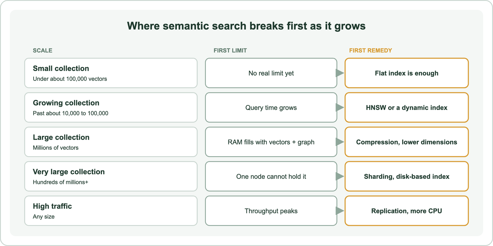
Memory is the limit that most teams hit first, so it deserves the most precise arithmetic.
Why does memory become the first limit when semantic search scales?
Memory becomes the first limit because an HNSW index keeps every vector and every graph connection in RAM, and both grow with the collection. Weaviate’s resource planning documentation puts it directly: memory determines the maximum supported dataset size, and it does not directly influence query speed. Only vectors are held in memory, not the original text.
The arithmetic is simple. A float32 vector uses 4 bytes per dimension. Weaviate’s example takes one million 384-dimensional vectors: 1,536 bytes each, about 1.5 GB in total. Its rule of thumb doubles that to 3 GB to cover the index and overhead. A finer estimate adds the graph. Each connection uses 8 to 10 bytes, so with maxConnections at 64 the estimate becomes one million times 1,536 bytes plus 640 bytes, about 2.2 GB.
Dimensions multiply everything. Weaviate’s best-practice guide estimates about 6 GB for one million 1024-dimensional vectors, but only 1.5 GB for 256 dimensions. At one hundred million items the same arithmetic reaches hundreds of gigabytes. That is why the guide calls choosing a lower-dimensional model the most effective single memory saving.
The calculator shows the graph staying the same size under compression, which matters at the next step. Memory pressure also changes which index makes sense.
How does the vector index choice change as a collection grows?
The vector index choice moves from a flat index for small collections to a graph index such as HNSW for large ones, and to a disk-based index when memory is the binding limit. Weaviate’s best-practice guide suggests a flat index when a collection will stay small, for example under 100,000 vectors. A flat index uses little memory but compares the query with every vector, so it slows as the collection grows.
HNSW fixes the speed problem. Malkov and Yashunin’s 2016 paper describes a multilayer proximity graph that a search descends from coarse to fine layers. Weaviate’s documentation says HNSW queries scale logarithmically with collection size. The cost is the in-memory graph, which grows with every vector.
Weaviate’s dynamic index bridges the two. It starts flat and converts to HNSW when a collection or tenant passes a threshold, 10,000 objects by default. The switch is one-way and needs asynchronous indexing. It suits multi-tenant systems where most tenants are small and a few grow large.
When RAM is the hard limit, disk-based indexes keep most data on SSD. Weaviate’s HFresh index keeps only a compressed centroid index in memory and stores posting lists on disk. The research behind this class of design is DiskANN. Subramanya and colleagues’ NeurIPS 2019 paper indexed one billion points on a single workstation with 64 GB of RAM and an SSD. On the SIFT1B dataset it served over 5,000 queries a second at under 3 milliseconds mean latency and over 95 percent 1-recall@1. Disk indexes trade some throughput for that memory saving. Compression offers a different trade.
How does vector compression reduce the cost of scaling?
Vector compression reduces the cost of scaling by storing each vector in fewer bits, which cuts memory sharply in exchange for a small loss of recall. Weaviate offers four methods. Its compression guide lists their typical memory savings: product quantization about 85 percent, scalar quantization 75 percent, 8-bit rotational quantization 75 percent, and binary quantization 97 percent.
| Method | Memory saved | Typical recall | Needs training |
|---|---|---|---|
| Rotational quantization, 8-bit | 75% (4x) | 98 to 99% | No |
| Scalar quantization | 75% | 95 to 97% | Yes |
| Product quantization | About 85% | Varies with settings | Yes |
| Binary quantization | 97% | Varies with data and model | No |
The table shows why Weaviate recommends 8-bit rotational quantization as a default: high recall, no training step, and a fourfold saving. Binary quantization saves the most but depends heavily on the embedding model.
Two caveats keep the estimate honest. First, quantization shrinks vectors, not the HNSW graph, so total memory falls less than the vector saving suggests. Second, Weaviate stores the uncompressed vectors on disk too, so disk use rises while RAM use falls. To recover recall, Weaviate over-fetches candidates using compressed vectors and rescores them with the uncompressed ones. Weaviate advises testing compression on your own data before production, because results depend on the embedding model. Once one machine is full even after compression, the collection has to spread out.
How do sharding and replication scale a semantic search cluster?
Sharding and replication scale a cluster in different directions: sharding splits data across nodes to hold more of it, while replication copies data to serve more queries and survive failures. Weaviate’s horizontal scaling documentation is explicit about what each does and does not improve.
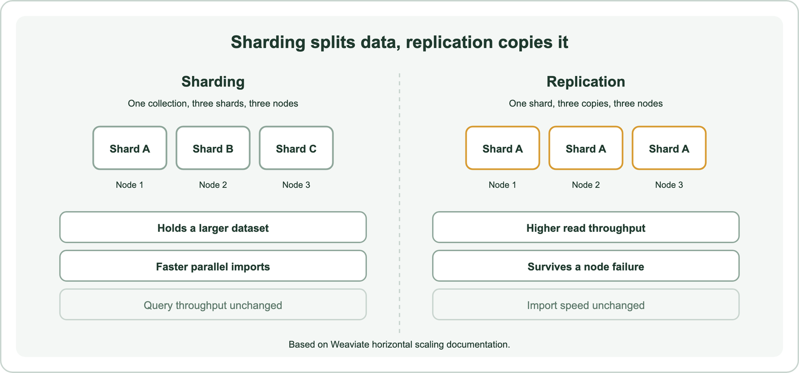
Each Weaviate shard holds its own vector index, inverted index, and object store. Adding shards across nodes lets a cluster hold a dataset no single machine could, and it speeds up imports because shards build in parallel. Weaviate notes that query throughput does not improve from more sharded nodes, since each query must visit every shard.
Replication works the other way. More replicas raise read throughput almost linearly and keep the service running when a node fails. Weaviate’s guidance also notes that replication allows rolling upgrades without downtime. Replicas do not speed up imports, because every copy must be written.
Plan shard count early. Weaviate warns that resharding is costly because of the HNSW structure, and it sets single-tenant shard count at collection creation. Multi-tenant collections place each tenant in its own shard, which isolates data and lets small tenants stay cheap. More machines raise capacity, but each query still has a latency budget.
How does query latency trade against recall at scale?
Query latency trades against recall through index settings: searching more of the graph finds more true neighbors but takes longer. In HNSW, the ef setting controls how many candidates a query explores. Weaviate’s resource guide explains that raising ef increases query time, while raising efConstruction increases import time without affecting queries.
Memory settings feed the same trade. Lowering maxConnections saves memory but reduces recall, and Weaviate suggests raising ef or efConstruction to compensate. Compression adds a third dial, because rescoring more candidates recovers recall at some speed cost. The recall versus latency trade-off covers how to tune these together.
Hardware choices follow the bottleneck. Weaviate’s FAQ notes that a single search runs on one thread, so more CPU cores raise throughput for parallel queries, not the speed of one query. Its rule: if throughput is the problem, add CPU; if response time is the problem, add memory so more data stays cached. Search latency breaks down where the rest of the time goes, and GPU acceleration for vector search covers when specialized hardware helps.
Recall can also degrade quietly. A faster setting that misses a few true neighbors may look fine in a demo and hurt users at scale. Measure recall against exact search on a sample after every tuning change. Writes create their own scaling costs.
Why are ingestion and re-embedding expensive at scale?
Ingestion and re-embedding become expensive at scale because every new item needs an embedding and a graph insertion, and every model change needs both again for the whole collection. Weaviate’s FAQ notes that imports are almost always CPU-bound because building the HNSW index is costly. Its suggestion is to favor CPU during bulk imports and memory during query-heavy periods.
Several operations touch every item. Changing the embedding model invalidates all stored vectors, because old and new vectors do not share a space. Every item must be embedded again and the index rebuilt. Enabling product quantization in Weaviate trains a codebook on 10,000 to 100,000 records per shard and makes the index read-only while it converts. Resharding moves data and rebuilds graphs.
Freshness adds steady load. A catalog or news collection that changes constantly keeps the index busy with inserts and deletes. Weaviate’s asynchronous indexing separates data ingestion from index building so writes do not stall. Real-time indexing and index freshness covers update patterns in depth.
The practical lesson is to treat model choice as a long-term commitment. Re-embedding one hundred million items costs inference for every item, plus index build time on every shard. Test a model thoroughly before the collection is large. These costs feed directly into capacity plans.
How should a team plan capacity for semantic search?
A team should plan capacity for semantic search by sizing memory from vector count and dimensions, choosing compression and index type, and only then deciding shards and replicas. Starting with machines before arithmetic usually buys the wrong resource.
A workable sequence has six steps:
- Estimate vector count and dimensions for the next year, not today.
- Calculate memory with the memory formula, including graph links.
- Test compression on a representative sample and record recall.
- Choose the index type for the size and memory budget.
- Set shard count for data size and replicas for throughput and availability.
- Load-test with real queries and measure latency and recall together.
The sequence puts cheap decisions before expensive ones. Hosting is the last big choice. Managed versus self-hosted search compares who runs the cluster, and the cost of semantic search covers how memory, compute, and storage turn into a bill. Both depend on the numbers from steps one to three.
Scaling semantic search means keeping retrieval fast, accurate, and affordable as the collection grows. Memory is usually the first limit, because an in-memory graph index holds every vector and connection. Compression cuts vector memory by 75 to 97 percent, disk-based indexes move most data to SSD, sharding spreads data across machines, and replication serves more queries. Each remedy trades something, usually recall, latency, or operational effort. The decision is to size memory with real arithmetic, test compression and index settings against measured recall, and add machines only for the limit the system has actually reached.