Home / Keyword search / TF-IDF Explained for Search

TF-IDF Explained for Search

TF-IDF is a term-weighting method that scores how important a word is to a document by multiplying how often the word appears in that document by how rare the word is across the collection. The first factor, term frequency, rewards documents that use a query word often. The second, inverse document frequency, rewards words that few documents contain, because a rare word says more about a document than a common one. Summing these weights over a query’s words gives a simple relevance score for keyword search. TF-IDF came out of research by Karen Spärck Jones, who proposed inverse document frequency in 1972, and Gerard Salton’s vector space work. It ranks well for its simplicity, but it lets repeated words add up without limit and handles document length crudely. BM25, which Weaviate uses for keyword search, keeps the same idea and fixes both problems.

What is TF-IDF in search?

TF-IDF in search is a way to weight each word in a document by combining how often it appears there with how rare it is across all documents. High weights mark words that are frequent in the document and unusual in the collection.

The intuition is easy to state. If a document mentions “refund” five times, it is probably about refunds. If nearly every document mentions “policy”, seeing “policy” in one more says little. TF-IDF captures both observations in one number per word and document.

The idea grew out of early information retrieval research. Karen Spärck Jones introduced inverse document frequency in her 1972 paper “A statistical interpretation of term specificity and its application in retrieval”. Gerard Salton and colleagues combined term weights with the vector space model, described in the vector space model.

TF-IDF serves two roles. In keyword search it scores documents against a query. In text analysis it turns documents into sparse vectors for clustering or classification. Both rely on the same weights, built from two factors that deserve a closer look. The broader context is in what is keyword search.

What does term frequency measure?

Term frequency measures how many times a word appears in a document, as a signal of how much the document is about that word. A document that repeats a word is assumed to focus on it.

The raw count is the simplest form. In the document “refund policy for refund requests”, the term frequency of “refund” is 2 and of “policy” is 1. Counting needs nothing more than the tokens produced by the analyzer, stored in the postings lists of the inverted index.

Raw counts overstate repetition. A document with ten mentions of a word is not ten times as relevant as one with a single mention. A common fix is sublinear scaling, using 1 plus the logarithm of the count, so each extra mention adds less. Weaviate’s 1.17 release notes make the same point about relevance: a term appearing three times in one document and six in another does not make the second twice as relevant.

Term frequency also favours long documents, which contain more words and so more chances to repeat any of them. Normalizing by document length reduces that bias. Neither fix addresses common words, which is the job of the second factor.

What does inverse document frequency measure?

Inverse document frequency measures how rare a word is across the collection, computed as the logarithm of the number of documents divided by the number of documents containing the word. Rare words get high values; words in every document get zero.

With N documents and a word appearing in df of them, the classic form is log(N / df). In a collection of four documents, a word in two of them has an IDF of log10(4 / 2), about 0.301. A word in three has log10(4 / 3), about 0.125. A word in all four has log10(1), which is 0, so it contributes nothing to any score.

The logarithm keeps IDF from growing too fast for very rare words. A word in one document out of four gets log10(4), about 0.602, which is double the value for a word in two documents. Without the logarithm, the ratio N / df would be 4 against 2, and very rare words would swamp every score in large collections.

Weaviate’s 1.17 release notes describe the same reasoning: if a term occurs rarely in the documents, then whenever it does occur, that occurrence is probably significant. IDF is the part of TF-IDF that also survives into BM25, explained in the BM25 algorithm. The two factors multiply into one weight.

How do you calculate TF-IDF step by step?

You calculate TF-IDF step by step by counting each query word in each document, multiplying by that word’s IDF, and summing over the query’s words. The highest sum ranks first.

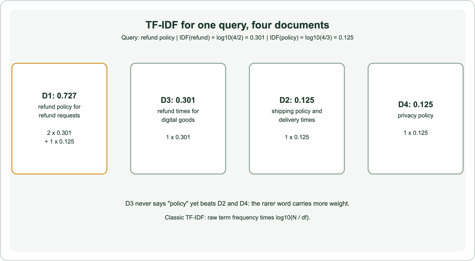
Four documents make up the collection. D1 is “refund policy for refund requests”, D2 “shipping policy and delivery times”, D3 “refund times for digital goods” and D4 “privacy policy”. “refund” appears in two documents, so its IDF is log10(4 / 2), about 0.301. “policy” appears in three, so its IDF is log10(4 / 3), about 0.125.

For the query “refund policy”, D1 scores 2 × 0.301 for refund plus 1 × 0.125 for policy, about 0.727. D3 has refund once and no policy: 0.301. D2 and D4 each have policy once and no refund: 0.125. The ranking is D1, D3, then D2 and D4 tied.

The result follows the intuition. D3 never says “policy” but beats two documents that do, because “refund” is the rarer and more informative word. The calculation was checked with a short script. Change the formula slightly, though, and the order can change.

How do TF-IDF variants change the ranking?

TF-IDF variants change the ranking because they differ in how they scale term frequency, smooth IDF and normalize for document length. There is no single TF-IDF formula, so the variant must be stated.

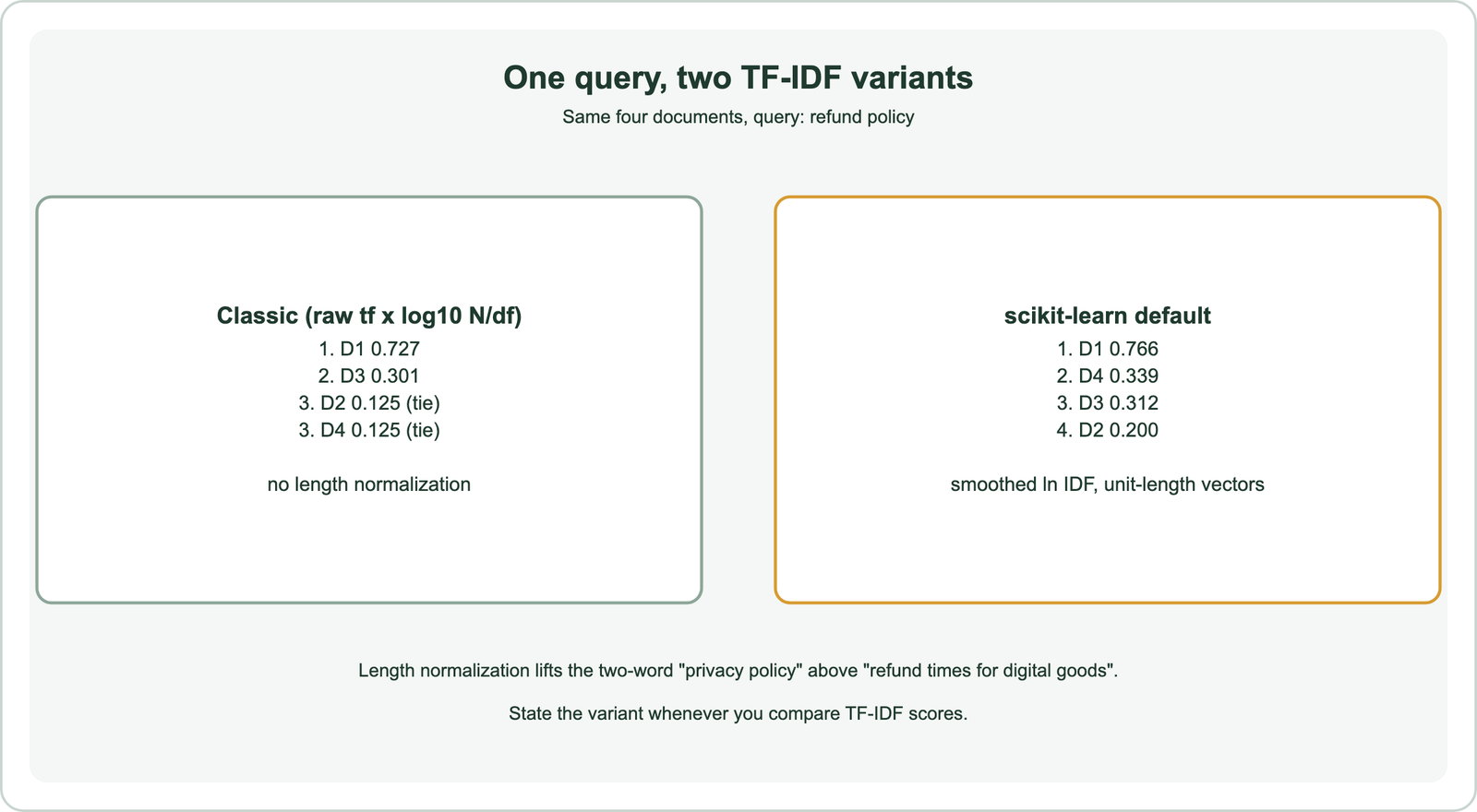
The scikit-learn library’s TfidfVectorizer is a common choice in Python. By default it smooths IDF as the natural logarithm of (1 + N) divided by (1 + df), plus 1, and scales each document vector to unit length. Its IDF for “refund” in the example is about 1.511, and for “policy” about 1.223.

Comparing the query vector with each document vector by cosine similarity gives D1 about 0.766, D4 about 0.339, D3 about 0.312 and D2 about 0.200. The two-word document “privacy policy” now beats “refund times for digital goods”, because length normalization gives each of its two words a large share of its vector.

Neither ranking is wrong; they encode different assumptions about length and repetition. That is the main practical lesson of TF-IDF: compare systems only with the same formula, and report which one you use. The values were computed with scikit-learn as a check. Both versions share weaknesses that BM25 was designed to fix.

What are the weaknesses of TF-IDF for ranking?

The weaknesses of TF-IDF for ranking are that term frequency rises without limit, length normalization is crude, and only exact word matches count. Each weakness distorts some rankings.

Unbounded term frequency lets a document that repeats a word many times dominate, even if it says little else. Sublinear scaling softens this but does not cap it. Keyword stuffing exploits exactly this behaviour.

Length handling is the second weakness. Without normalization, long documents win because they contain more words. With full normalization, as the scikit-learn example shows, very short documents can win because each word takes a large share. Neither extreme matches how relevance actually varies with length.

The third weakness is shared with all keyword methods. TF-IDF only sees the words that are present. “Cancel subscription” scores zero against “end membership” no matter how the weights are tuned, a problem covered in the vocabulary mismatch problem. The first two weaknesses are what BM25 addresses.

How does BM25 improve on TF-IDF?

BM25 improves on TF-IDF by saturating term frequency, so repeated words add less and less, and by normalizing for document length relative to the average, with tunable strength. It keeps IDF at its core.

Weaviate’s 1.17 release notes describe TF-IDF as the ranking function upon which BM25 builds, refined to codify retrieval intuitions such as diminishing returns from repetition. The k1 parameter controls how quickly term frequency saturates, and the b parameter controls how strongly document length counts. Weaviate’s academy course gives their defaults as 1.2 and 0.75.

The result is a scoring function that rarely needs tuning and behaves sensibly across short and long documents. It became the standard keyword ranking function, and Weaviate uses BM25F, a version that weights several fields separately, for its keyword search. The formula and parameters are covered in the BM25 algorithm.

TF-IDF remains useful outside ranking. As a sparse vector representation it supports clustering, classification and quick baselines. Learned sparse models such as SPLADE replace hand-set weights with learned ones while keeping the same sparse form, as described in sparse retrieval. Code makes the comparison concrete.

How do you compute TF-IDF scores in Python?

You compute TF-IDF scores in Python either with a few lines of standard-library code for the classic formula or with scikit-learn’s TfidfVectorizer for its smoothed, normalized variant. Both were run on the example as a check.

import math, re
from collections import Counter

docs = {"D1": "refund policy for refund requests",
        "D2": "shipping policy and delivery times",
        "D3": "refund times for digital goods",
        "D4": "privacy policy"}
tok = lambda s: re.findall(r"[a-z]+", s.lower())
N = len(docs)
df = Counter(t for text in docs.values() for t in set(tok(text)))

def tfidf_score(query, text):
    tf = Counter(tok(text))
    return sum(tf[t] * math.log10(N / df[t]) for t in tok(query) if df[t])

for name, text in docs.items():
    print(name, round(tfidf_score("refund policy", text), 3))   # D1 0.727, D2 0.125, D3 0.301, D4 0.125

The function counts each query word in the document and multiplies by its IDF. Words absent from the collection are skipped, since their document frequency is zero. With scikit-learn, fitting a TfidfVectorizer on the four documents and taking the dot product of each document vector with the transformed query gives the cosine scores from the variants section.

For production keyword search, use the engine’s built-in ranking rather than hand-rolled TF-IDF. Search engines such as Weaviate apply BM25 over the inverted index with stemming, stopwords and field weights already handled, as described in full-text search. Word-form handling is covered in stemming and lemmatization.

TF-IDF weights a word by how often it appears in a document times how rare it is across the collection, so rare, repeated query words rank documents highest. In the worked example, the rare word “refund” lifts D1 to 0.727 and D3 to 0.301 above documents with only the common word “policy”. Variants change the order, as scikit-learn’s normalized version shows by lifting a short document, so always state the formula. TF-IDF’s unbounded term frequency and crude length handling led to BM25, which keeps IDF and adds saturation and length normalization, and which Weaviate uses for keyword search.