Home / Scale and cost / Semantic Search Latency: Where the Milliseconds Go

Semantic Search Latency: Where the Milliseconds Go

Semantic search latency is the time from receiving a query to returning results. It is the sum of several stages: embedding the query, searching the vector index, running keyword search and fusion, fetching objects, reranking and, in RAG, generating an answer. The vector index is rarely the slow part. Weaviate’s published ANN benchmark reports mean latencies of a few milliseconds for unfiltered top-10 queries over collections of 1 to 10 million vectors. Those figures include network time and object retrieval. Calling a hosted embedding API, reranking dozens of candidates with a cross-encoder, or generating an answer with a language model usually costs far more. Reducing latency starts with measuring each stage separately. Then cut the slowest: cache query embeddings, tune the index, rerank fewer candidates, return smaller payloads and stream generated answers.

What is search latency?

Search latency is the elapsed time between a search request and its response, usually reported as a mean and as percentiles such as p95 or p99. It is different from throughput, the number of queries served per second.

Weaviate’s benchmark documentation explains the distinction. A mean latency of 5 milliseconds says a single request takes 5 milliseconds on average, but not how many requests the system can handle at once. If a server handled one query at a time, its throughput would be roughly 1 second divided by the mean latency. Real systems serve many requests concurrently, so throughput must be measured, not derived.

Percentiles show the tail. A p99 latency is the time within which 99 out of 100 requests finish; the remaining 1 percent are slower. Users notice slow outliers, and service agreements are often written as a throughput at a given percentile latency. Track both the mean and a high percentile. Tail latency often comes from a few causes that the mean hides, such as cold caches after a restart, garbage collection pauses, very selective filters or an overloaded node.

Where does the time go in a semantic search request?

The time in a semantic search request goes into six stages: embedding the query, vector search, keyword search and fusion, fetching objects, reranking and, for RAG, generation. Their costs differ by orders of magnitude.

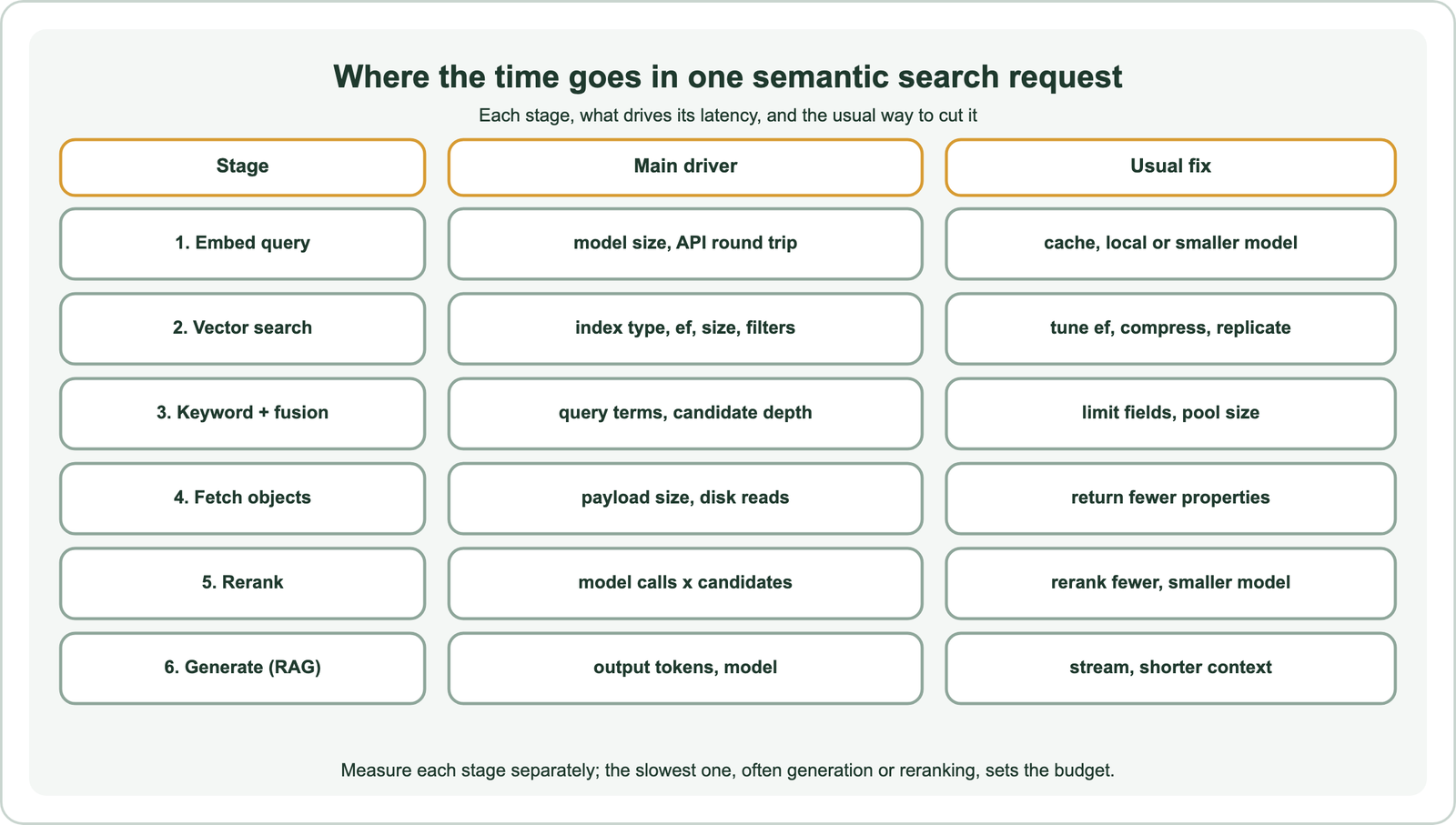
Query embedding is a model call. With a hosted API it includes a network round trip; with a local model it depends on model size and hardware. Vector search walks the index, keyword search reads the inverted index, and fusion merges the two. Fetching returns the matched objects, which grows with the number and size of properties requested.

Reranking and generation are usually the heaviest. A cross-encoder reranker runs the model once per candidate, so 50 candidates means 50 pair evaluations. A language model generates an answer token by token, and long answers take seconds. Reranking latency and cost covers the reranking side in detail.

How fast is vector search itself?

Vector search itself is typically fast, measured in milliseconds on a well-sized index, as Weaviate’s published ANN benchmark shows for collections of 1 to 10 million vectors. Its speed depends on recall settings, filters and hardware.

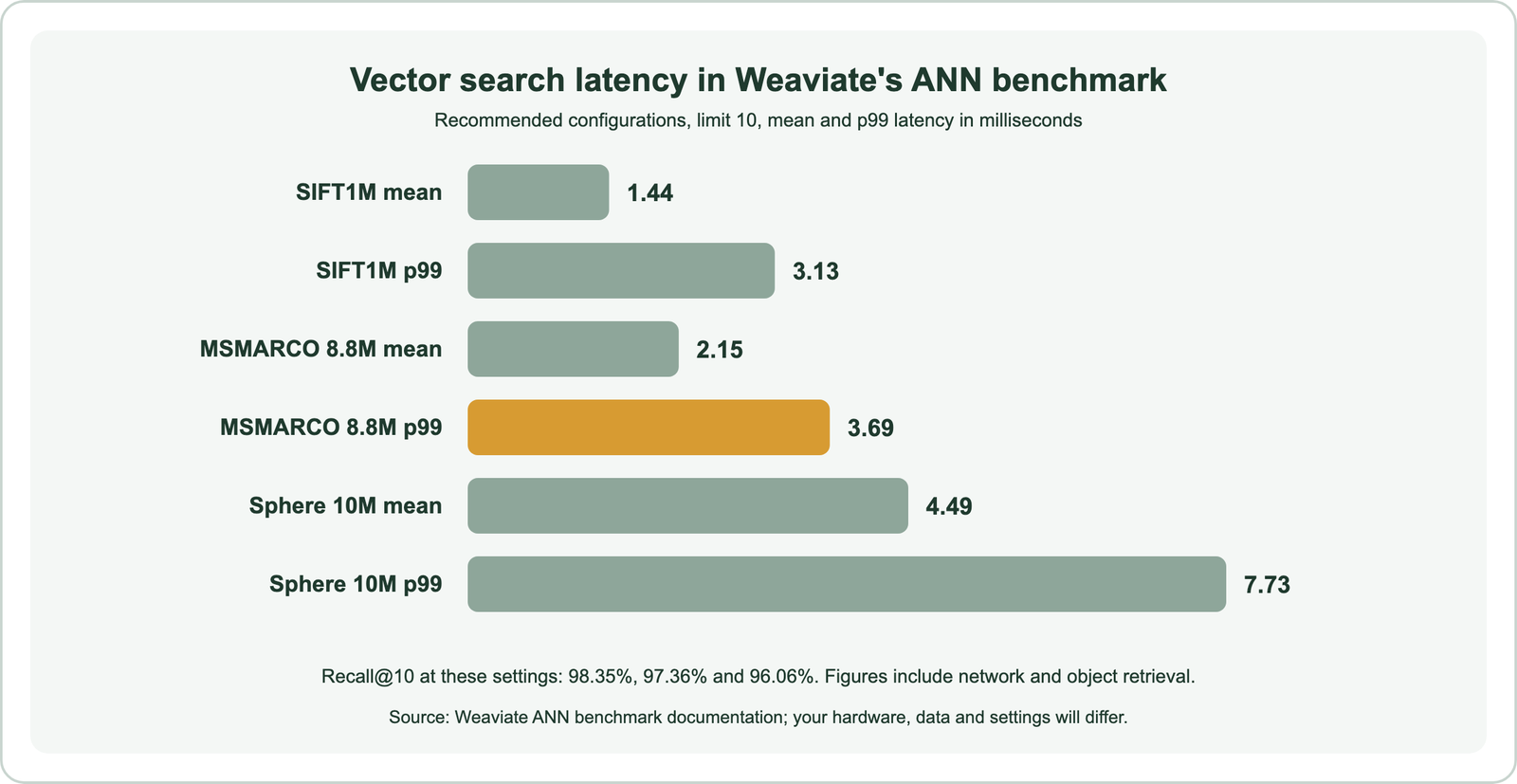
Weaviate’s recommended configurations report 1.44 milliseconds mean and 3.13 p99 on SIFT1M at 98.35 percent recall at 10. On 8.8 million MS MARCO vectors they report 2.15 and 3.69 milliseconds at 97.36 percent recall, and on 10 million Sphere vectors 4.49 and 7.73 at 96.06 percent. Each request includes network time and fetching the objects from disk. The benchmark is open source, so the same tests can be run on your own hardware.

Raising recall costs time. HNSW’s ef setting widens the search, and Weaviate’s documentation notes diminishing recall gains above 512. The recall vs latency trade-off covers tuning, and exact vs approximate search explains why approximate indexes are needed at all.

How do filters, hybrid search and compression affect latency?

Filters, hybrid search and compression all change latency: restrictive filters can slow graph search, hybrid adds a keyword leg and fusion, and compression usually speeds up search while rescoring adds a little back. Measure each on your own queries.

When a filter matches few objects, walking an HNSW graph becomes inefficient. Weaviate switches to a flat scan of the matching objects when fewer than a cut-off match, 40,000 objects by default, and offers filter strategies such as ACORN, the default from version 1.34. Hybrid queries run BM25 and vector search in parallel, then fuse, so their cost is roughly the slower leg plus fusion. Larger candidate pools improve fusion quality but cost time.

Compression shrinks vectors, so more fit in memory and distance calculations run faster. Weaviate’s 8-bit rotational quantization blog reports throughput gains with little recall loss. Rescoring with uncompressed vectors restores recall at some cost. Embedding quantization covers the methods.

How do you measure search latency?

You measure search latency by timing each stage separately under realistic load, and by using the database’s own tools to break down slow queries. End-to-end numbers alone hide the cause.

Instrument the application so every request logs the time for embedding, search, reranking and generation. Run load tests with production-like concurrency, because latency grows as concurrent requests queue. Weaviate exposes Prometheus metrics for query latency and request rates, logs slow queries above a configurable threshold, and offers query profiling with per-shard timings. The profiles separate vector search, keyword scoring and filter evaluation.

Report p50, p95 and p99 alongside the mean, and keep the test queries fixed so changes are comparable. Note the hardware and settings with each result. Weaviate’s benchmark FAQ warns that single-thread results cannot be scaled up to predict multi-threaded throughput, because locks and contention do not scale linearly.

How do you reduce semantic search latency?

You reduce semantic search latency by attacking the slowest stage first: caching or speeding up query embedding, tuning the index, reranking fewer candidates, trimming payloads and streaming generated answers. Small changes to heavy stages beat large changes to light ones.

Cache embeddings for repeated queries, and consider a semantic cache that reuses answers for near-identical questions. Run a smaller embedding model close to the database to avoid a network round trip. Tune ef to the lowest value that meets your recall target. Request only the properties the interface needs.

For reranking, pass fewer candidates or use a smaller model. For RAG, stream tokens so users see text immediately, and keep the context short. Add replicas when concurrency, rather than single-query speed, is the problem; Weaviate’s documentation notes that replication raises query throughput nearly linearly. Scaling semantic search covers capacity planning.

How does latency add up in RAG and agent workflows?

Latency adds up in RAG and agent workflows because each answer can involve several searches and model calls in sequence, so per-step delays multiply. A fast search inside a slow loop is still slow.

A basic RAG answer runs one search and one generation. Query rewriting adds a model call before the search, and reranking adds one after. An agent may plan, search, read, search again and then answer, repeating the full search pipeline several times. If each round costs a model call plus a search, the total grows with the number of rounds, and the user waits for all of them.

Three habits help. Run independent searches in parallel instead of one after another. Cap the number of agent steps and stop early when the evidence is sufficient. Stream partial results, such as the sources found so far, while the final answer is generated. Agentic retrieval and agentic search covers these workflows in more depth.

What trade-offs does lower latency require?

Lower latency usually requires trading against recall, cost or answer quality, so latency targets should be set together with quality and budget targets. The fastest system is rarely the best one.

Lowering ef or compressing harder speeds search but can miss true neighbours. Reranking fewer candidates saves time but can drop the best result. Smaller embedding or language models are faster but may understand queries less well. More replicas or GPUs cut latency at a higher bill, as covered in the cost of semantic search and GPU acceleration for vector search.

Write the targets down: for example a p95 for the search step, a separate one for full RAG answers, a minimum recall and a monthly budget. Then tune against all of them on the same test set. Index freshness, covered in real-time indexing and index freshness, and hosting, covered in managed vs self-hosted search, also shape what is achievable.

Semantic search latency is the sum of its stages: query embedding, vector search, keyword search and fusion, object fetching, reranking and generation. The vector index is often the fastest part; Weaviate’s ANN benchmark reports mean latencies of 1.44 to 4.49 milliseconds on 1 to 10 million vectors. Embedding API calls, reranking and generation usually dominate. Measure each stage under load with percentiles, then cut the slowest: cache, tune the index to a recall target, rerank less, trim payloads and stream answers. Set latency targets together with recall and budget.