Home / How it works / Cosine Similarity vs Dot Product vs Euclidean (L2) Distance
ExplainerCosine Similarity vs Dot Product vs Euclidean (L2) Distance
Cosine similarity, dot product, and Euclidean (L2) distance measure how close two vectors are: cosine by direction, dot product by direction and length, and L2 by straight-line gap. In semantic search, they decide which stored embeddings count as nearest to a query. They often rank results the same way, but not always. When vectors are normalized to length 1, all three produce identical rankings, because each one becomes a simple function of the angle between the vectors. When vectors have different lengths, the dot product rewards longer vectors and L2 penalizes distant ones, so the order can change. The safe rule is to use the metric the embedding model was trained with. Most text embedding models use cosine, which is also Weaviate’s default.
Distance metrics in four facts
- Cosine distance is one minus cosine similarity and ranges from 0 for identical directions to 2 for opposite ones.
- For unit-length vectors, squared L2 distance equals 2 minus 2 times cosine similarity.
- On normalized vectors, cosine, dot product, and L2 give the same ranking of results.
- The search metric should match the metric the embedding model was trained with.
What is the difference between cosine similarity, dot product, and Euclidean distance?
The difference is what each metric measures: cosine similarity measures the angle between vectors, the dot product measures angle and length together, and Euclidean distance measures how far apart the vector tips are. All three compare the same two lists of numbers. They just summarize them differently.
| Metric | Formula | Range | Higher means | Sensitive to length |
|---|---|---|---|---|
| Cosine similarity | a·b / (|a| |b|) | −1 to 1 | More similar | No |
| Cosine distance | 1 − cosine similarity | 0 to 2 | Less similar | No |
| Dot product | Σ aᵢ bᵢ | Unbounded | More similar | Yes |
| Euclidean (L2) | √Σ (aᵢ − bᵢ)² | 0 and up | Less similar | Yes |
The table shows two families. Cosine similarity and the dot product are similarities, where bigger numbers mean closer. Cosine distance and L2 are distances, where smaller numbers mean closer. Mixing the two directions is the most common source of confusion when reading scores.
Length is the other split. Cosine ignores how long the vectors are, so a short text and a long text about the same topic can score as identical. The dot product and L2 both react to length. Whether that helps depends on what length means for a given model. Each metric is easier to judge once its arithmetic is clear, starting with cosine.
How is cosine similarity calculated?
Cosine similarity is calculated by dividing the dot product of two vectors by the product of their lengths, which gives the cosine of the angle between them. The result runs from 1 for the same direction, through 0 for perpendicular, to −1 for opposite directions.
A small worked example shows the steps. Take a = (1, 2, 2) and b = (2, 1, 2). The dot product is 1×2 + 2×1 + 2×2 = 8. Each vector has length √(1 + 4 + 4) = 3. Cosine similarity is 8 / (3 × 3) = 0.889. The vectors point in nearly the same direction.
Cosine distance flips the scale so smaller means closer. Weaviate’s distance reference defines it as one minus cosine similarity, with a range from 0 for identical vectors to 2 for opposing ones. In the example, cosine distance is 1 − 0.889 = 0.111.
Cosine is popular for text because it ignores length. Weaviate’s blog on distance metrics gives the intuition: if a word appears 30 times in one document and 10 in another, the counts differ in size, but the documents can still point the same way. The metric calculator tests any pair of vectors. The dot product, by contrast, keeps the length information.
How does the dot product measure similarity?
The dot product measures similarity by multiplying matching dimensions and adding the results, so it grows when vectors point the same way and when they are long. It equals the length of a, times the length of b, times the cosine of the angle between them.
That formula explains the difference from cosine. Cosine is the dot product with the lengths divided out. The dot product keeps them. If a model encodes something useful in vector length, such as confidence or popularity, the dot product uses it. If length is noise, the dot product lets it distort the ranking.
The dot product has no fixed range. It can be any positive or negative number, so its values are hard to read without context. Weaviate’s distance reference notes that the dot product is a similarity rather than a distance. Weaviate therefore returns the negative dot product, so smaller values still mean more similar, as with every other metric it offers.
The dot product is also the cheapest to compute: one multiply and one add per dimension. That is why some systems normalize vectors once at indexing time and then use the dot product. Weaviate’s reference says it does exactly this for cosine: it normalizes vectors to length 1 and computes the dot product for efficiency. The relevance scores guide covers how to interpret the resulting numbers. L2 distance takes a different view of the same vectors.
What is L2 distance, and how is it calculated?
L2 distance, also called Euclidean distance, is the straight-line distance between the tips of two vectors, calculated as the square root of the sum of squared differences between matching dimensions. It is the everyday notion of distance, extended to any number of dimensions.
The formula is √Σ(aᵢ − bᵢ)². In the earlier example, the differences are −1, 1, and 0. Their squares sum to 2, so the L2 distance is √2, about 1.414. Many systems skip the square root and use squared L2 instead. Weaviate’s l2-squared metric is defined as Σ(aᵢ − bᵢ)², with a range from 0 for identical vectors upward. Dropping the root saves work and never changes which item is nearest.
The name L2 comes from the L2 norm, the vector length used in the formula. A vector’s Euclidean length is the L2 norm of the vector itself. Normalized Euclidean distance usually means L2 distance computed after each vector has been scaled to length 1. That turns L2 into a pure measure of direction.
Unlike cosine, L2 has no similarity form, and Weaviate’s search documentation notes that Euclidean distance is only expressible as a distance. Two vectors in the same direction but of different lengths have a cosine distance of 0 and a positive L2 distance. That gap closes completely once vectors are normalized.
Why do the metrics agree on normalized vectors?
The metrics agree on normalized vectors because, once every vector has length 1, the dot product equals cosine similarity and squared L2 distance equals 2 minus 2 times cosine similarity. All three become functions of the same angle, so they order results identically.
The identity follows from expanding the L2 formula. Squared L2 equals |a|² + |b|² − 2a·b. With both lengths equal to 1, that becomes 2 − 2a·b, and a·b is the cosine. In the worked example, normalizing gives a cosine of 0.889, so squared L2 is 2 − 2 × 0.889 = 0.222. The calculator’s last row shows the same result for any pair you enter.
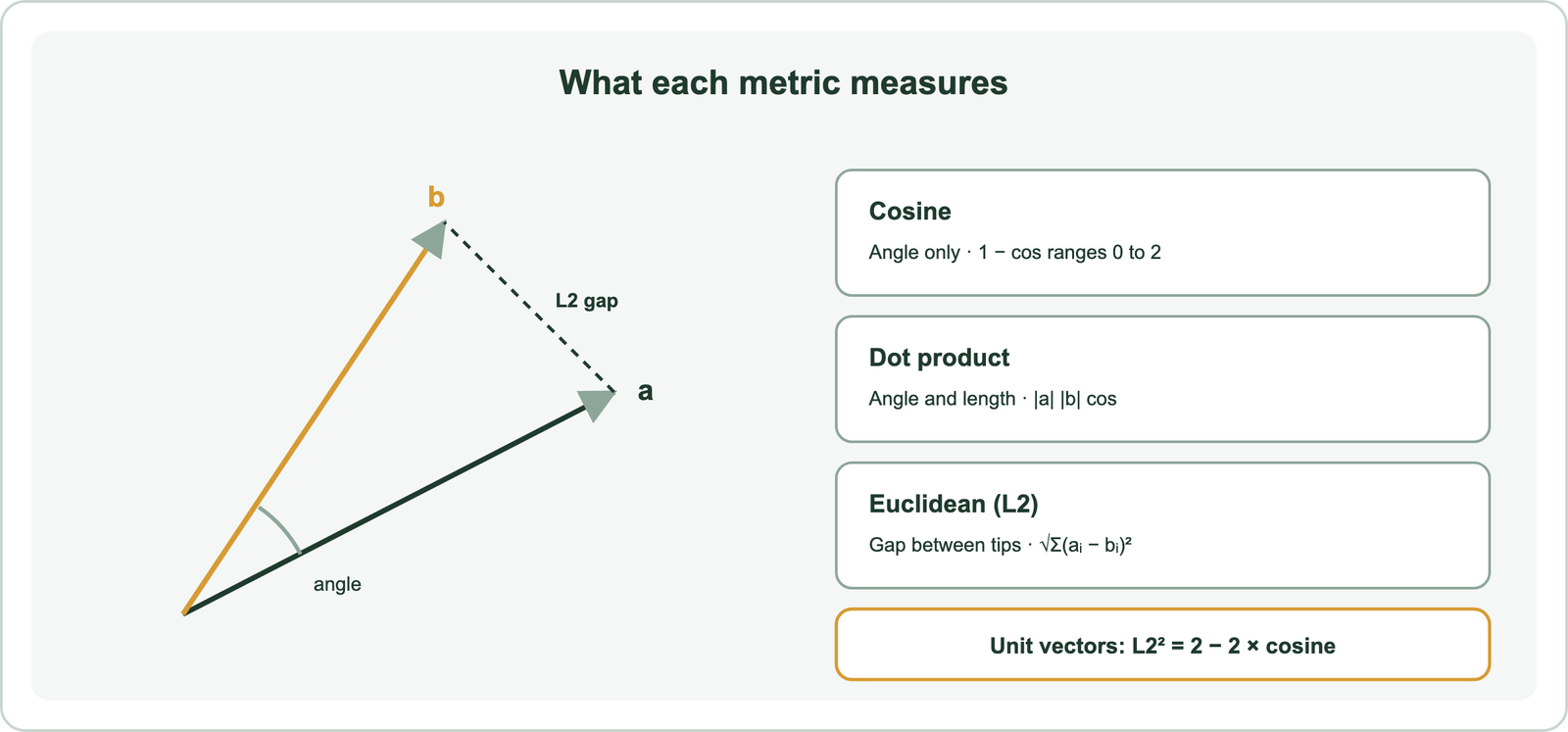
Weaviate’s distance metrics article states the practical version: if data is normalized, cosine and dot product are exactly the same. Many embedding models already return normalized vectors, which is why switching among the three often changes nothing.
The agreement breaks when lengths vary. Then a long vector can top a dot-product ranking while a closer, shorter one tops the L2 ranking. Checking whether your model’s vectors have length 1 settles which case you are in. Two further metrics complete the picture.
How do Manhattan and Minkowski distance relate to L2 distance?
Manhattan and L2 distance are both special cases of Minkowski distance, which raises each absolute difference to a power p, sums them, and takes the p-th root. With p = 1 it gives Manhattan distance, and with p = 2 it gives Euclidean distance.
Manhattan distance, also called L1 or taxicab distance, adds up absolute differences along each axis. Weaviate added it as the manhattan metric in version 1.15. Its release notes give a worked example: comparing [1, 9, 3, 4, 5] with [1, 2, 3, 9, 5] gives 0 + 7 + 0 + 5 + 0 = 12. The same release added Hamming distance, which counts dimensions that differ, giving 2 for those vectors.
Weaviate’s distance metrics article describes an accuracy versus speed trade-off between L1 and L2. L1 avoids squaring, and the article points to research by Aggarwal and colleagues on how distance metrics behave as dimensions grow. Higher Minkowski orders weight the largest single difference more heavily, and very large p approaches the maximum difference on any one axis.
Weaviate’s distance reference also notes that its SIMD hardware speed-ups cover cosine, dot, and L2-squared but not Manhattan or Hamming. For text embeddings, the practical choice almost always comes down to the first three. Picking among them depends on the model.
Which distance metric should semantic search use?
Semantic search should use the distance metric the embedding model was trained with, which for most text embedding models is cosine. Weaviate’s vector search documentation states that each vectorizer model is trained with a specific metric and that search should use the same one.
The model card usually says which one. Weaviate’s vector database guide gives examples: OpenAI documents cosine similarity for its ada-002 embeddings, and some MiniLM models on Hugging Face support cosine, dot product, and Euclidean distance. Weaviate uses cosine as its default because it is the typical metric for vectorizer models.
A short checklist settles the choice:
- Read the model card for its training metric.
- Check whether the model returns normalized vectors.
- Use cosine or dot product for normalized vectors; both rank identically.
- Use the documented metric exactly when vectors are not normalized.
- Confirm the index supports it; Weaviate’s HFresh index supports only cosine and L2-squared.
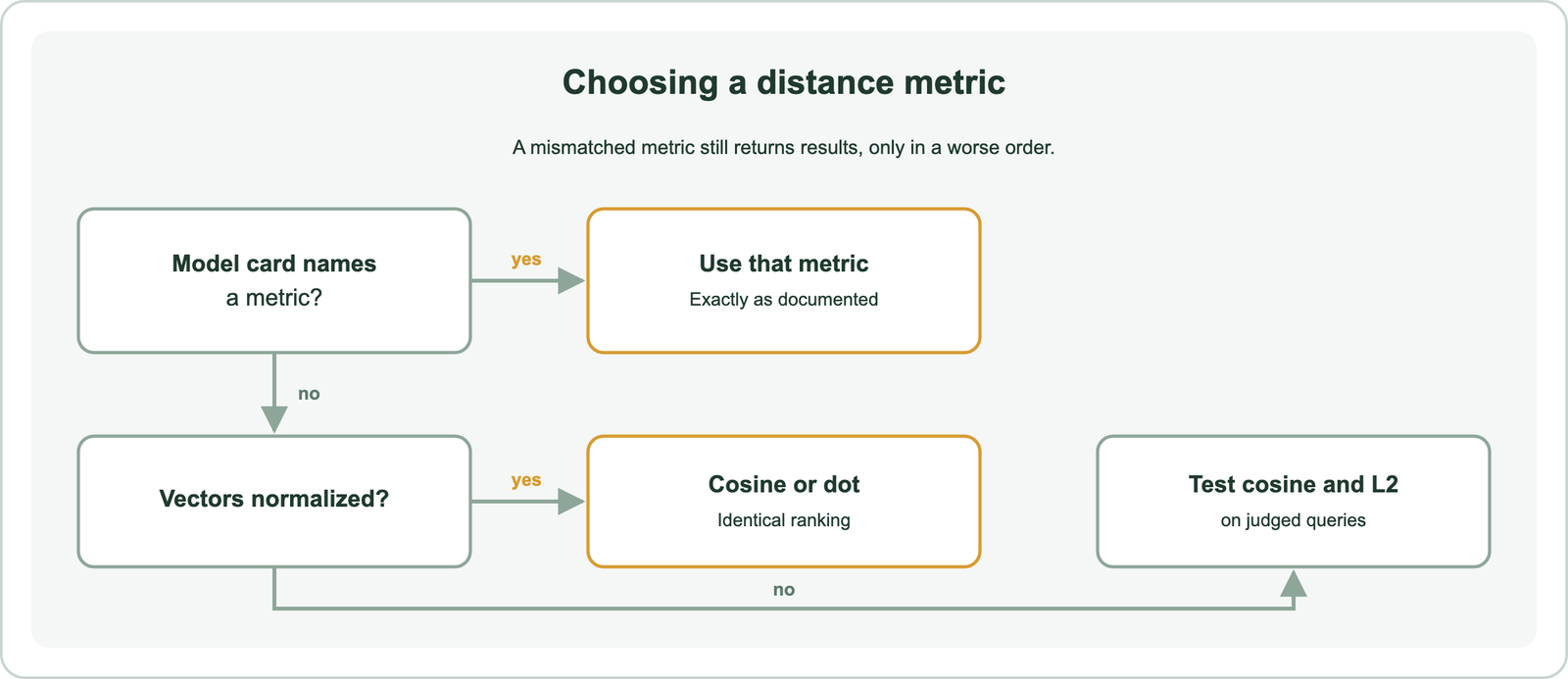
The checklist avoids a silent failure: a mismatched metric still returns results, just in a worse order. The metric is set when the index is created, as described in semantic indexing and vector indexes, and changing it later means rebuilding. The numbers it produces also need care when shown to users.
How do vector databases report distance and similarity?
Vector databases report either a distance, where lower is closer, or a similarity, where higher is closer, and the scale depends on the metric and the database. The same pair of vectors can show 0.111 in one system and 0.889 in another.
Weaviate reports distances for all its metrics. Its reference states that larger distance values always mean lower similarity. That is why it negates the dot product: a dot product of 3 becomes a distance of −3, which ranks ahead of −2. A query can also use a distance as a cutoff, returning only results closer than a chosen value.
Thresholds do not transfer between metrics or models. A cosine distance of 0.3 has no fixed meaning in L2 terms, and different models spread their vectors differently. Choose cutoffs from judged examples on your own data. Top-k retrieval covers count-based cutoffs, and similarity search and vector search explain where these scores come from.
The metric is one setting among many in the system. The semantic search pipeline shows where it fits, and approximate nearest neighbor search, exact versus approximate search, and semantic search architecture cover the index around it. The vectors themselves are covered in dense vectors, sparse vectors, and dense versus sparse vectors. Related matching topics include semantic matching, synonyms and related terms, multilingual and cross-lingual search, and chunking for semantic search.
Cosine similarity, dot product, and Euclidean (L2) distance measure how close two vectors are by angle, by angle and length, and by straight-line gap. On normalized vectors, the identity squared L2 = 2 − 2 × cosine makes all three rank results identically. When lengths vary, they can disagree, and Manhattan and Minkowski distance add further options with their own trade-offs. The decision is simple: use the metric the embedding model was trained with, check whether its vectors are normalized, and set any score cutoffs from judged results rather than from numbers copied across systems.