Home / Foundations / The Vector Space Model of Information Retrieval

The Vector Space Model of Information Retrieval

The vector space model represents every document and query as a vector with one dimension per vocabulary term. It weights each term by how informative it is and ranks documents by the cosine of the angle between their vector and the query’s. Developed by Gerard Salton and colleagues around the SMART retrieval system and set out in a 1975 paper with Wong and Yang, it replaced yes-or-no Boolean matching with graded relevance scores. Its usual weighting, TF-IDF, rewards terms that appear often in a document but rarely across the collection. The model’s vectors are sparse, mostly zeros, and two texts only match if they share terms, which is the vocabulary mismatch problem. Later methods kept its central idea, documents as vectors compared by similarity, but changed what the dimensions mean: latent semantic indexing compressed terms into topics, and neural embeddings learned dense dimensions of meaning. Weaviate’s hybrid search still combines the two descendants: BM25 sparse scoring and dense vector search.

What is the vector space model?

The vector space model is an information retrieval model that places documents and queries as vectors in a space whose dimensions are the terms of the vocabulary, and measures relevance as closeness in that space. It is the conceptual ancestor of modern vector search.

Before it, many retrieval systems used Boolean logic. A query such as “pie AND recipe” either matched a document or did not, and matches came back unranked. Users had to craft precise queries and sift through unordered results. The vector space model changed this by scoring every document, so results could be ranked from most to least relevant.

The idea is geometric. If each term is an axis, a document is a point, or an arrow from the origin, whose coordinates are its term weights. Documents about similar subjects use similar terms, so their arrows point in similar directions. A query is turned into a vector the same way, and the closest documents by angle come first.

That framing, documents as vectors and relevance as similarity, carried forward into every later retrieval model. The broader field is introduced in what is information retrieval.

Who is credited with developing the vector space model?

The vector space model was developed by Gerard Salton and colleagues, chiefly at Cornell University, through the SMART retrieval system and their 1975 paper “A Vector Space Model for Automatic Indexing”. Salton is often called a father of information retrieval.

The SMART system, built from the 1960s onward, was a laboratory for testing retrieval ideas on real document collections with relevance judgements. Term weighting, relevance feedback and the vector model itself were refined there. The 1975 paper by Salton, Wong and Yang, published in Communications of the ACM, framed indexing as choosing term weights that spread documents well in the vector space.

Inverse document frequency, the “IDF” in TF-IDF, came from Karen Spärck Jones in 1972, who showed that rare terms are better discriminators than common ones. Combined with term frequency, it became the standard weighting for vector space retrieval and the root of later scoring functions such as BM25.

Relevance feedback was another SMART idea built on the same geometry. If a user marks some results as relevant, the query vector can be moved towards those documents and away from irrelevant ones, a method associated with Rocchio. The refined query then finds more documents like the good ones. Modern systems still use versions of this, from query expansion to recommendations based on items a user liked.

How are documents turned into vectors?

Documents are turned into vectors by counting each vocabulary term in the document and weighting the counts, most often with TF-IDF, which multiplies term frequency by inverse document frequency. Terms that are absent get a weight of zero.

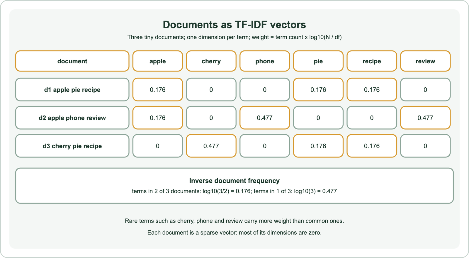
Term frequency rewards repetition: a document that mentions “recipe” five times is probably more about recipes than one that mentions it once. Inverse document frequency rewards rarity: a term that appears in every document distinguishes nothing, while one that appears in few documents is a strong signal. In the toy collection, “apple”, “pie” and “recipe” each appear in two of three documents and get 0.176, while “cherry”, “phone” and “review” appear in one and get 0.477.

Real vocabularies have tens of thousands of terms, so each document vector has that many dimensions, nearly all zero. These are sparse vectors, a term described in sparse vectors. The detailed formula and its variants are covered in TF-IDF.

How does the vector space model rank documents?

The vector space model ranks documents by cosine similarity: the dot product of the query and document vectors divided by the product of their lengths, which depends on direction rather than magnitude. The highest cosine ranks first.

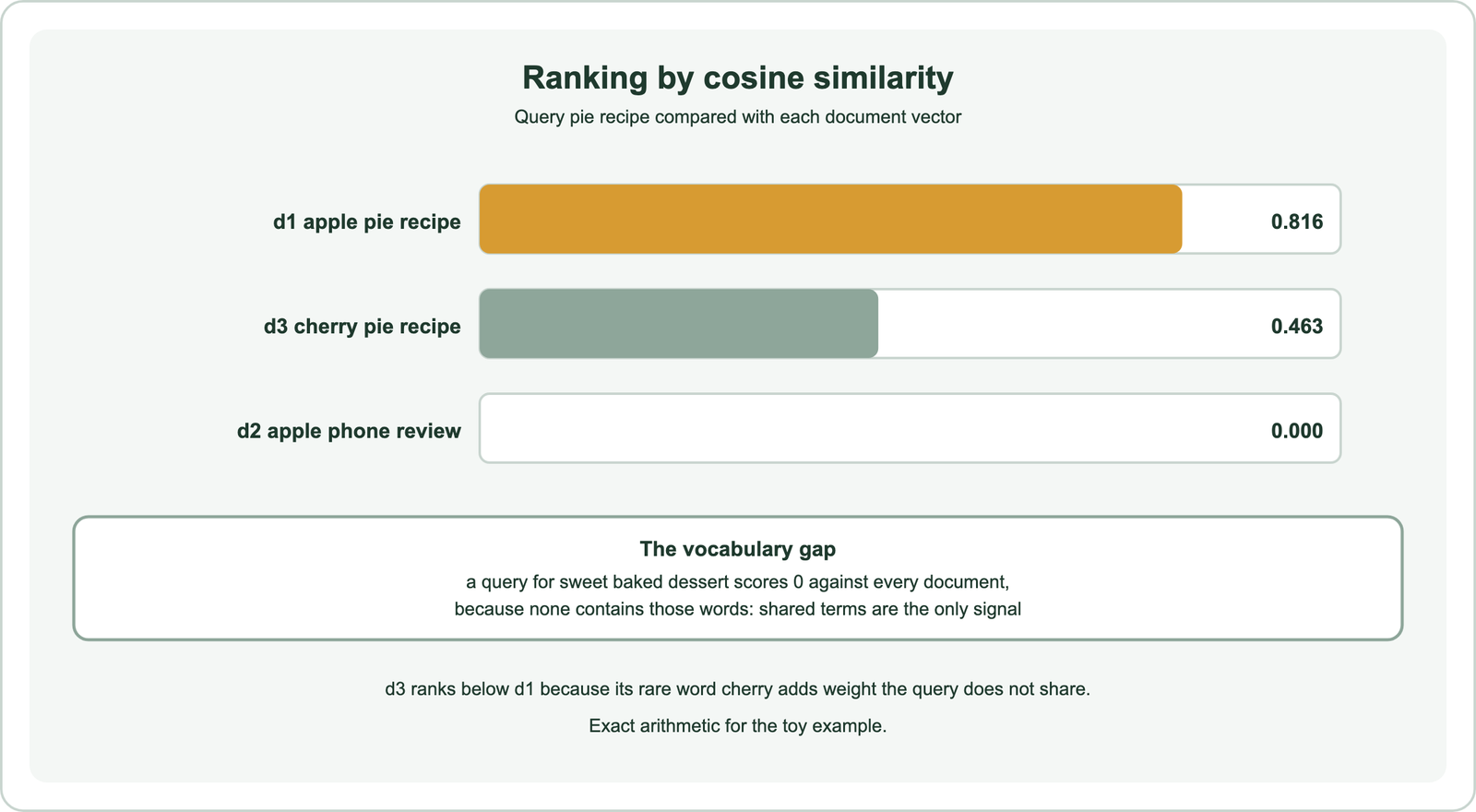
Cosine similarity normalises for length. A long document has a longer vector simply because it has more words; dividing by the vector lengths removes that advantage, so a short, focused document can outrank a long, rambling one. The measure and its relatives are compared in cosine vs dot product vs Euclidean distance.

The toy example shows the mechanics and a quirk. The query “pie recipe” scores 0.816 against “apple pie recipe” and 0.463 against “cherry pie recipe”, although both match the query equally well. The rare word “cherry” carries a high weight that the query does not share, which lengthens d3’s vector and lowers its cosine. “Apple phone review” shares no query terms and scores 0.

What are the limits of the vector space model?

The vector space model’s main limits are that it matches only shared terms, treats terms as independent, ignores word order and needs a weighting scheme tuned by hand. The first limit is the most important for search.

Shared terms are its only signal. A query for “sweet baked dessert” scores zero against “cherry pie recipe”, because no words overlap. Synonyms, paraphrases and related concepts are invisible. This is the problem described in the vocabulary mismatch problem.

Each term is also treated as its own independent axis. “Car” and “automobile” are as unrelated as “car” and “banana”, and word order is ignored, so “dog bites man” and “man bites dog” get the same vector. Term weights and normalisation had to be designed and tuned, which motivated probabilistic models and, later, BM25.

How does the vector space model connect to embeddings?

The vector space model connects to embeddings by establishing documents as vectors compared by similarity, after which later methods replaced its term dimensions with learned dimensions of meaning. The retrieval step stayed recognisably the same.

Latent semantic indexing, from 1990, compressed the term-document matrix into a few hundred latent topics, so related terms could share dimensions; it is covered in latent semantic indexing. Word2vec and GloVe learned dense word vectors from context, described in word2vec and GloVe. Transformers and sentence embedding models then produced dense vectors for whole passages, covered in transformers and BERT in search and Sentence-BERT.

Meanwhile, the sparse branch evolved into BM25. Weaviate’s hybrid search article describes BM25 as building on TF-IDF and adding a normalisation penalty for document length relative to the average. Its BlockMax WAND article describes IDF as the measure of term importance that, combined with term frequency, became the cornerstone of keyword search. Both branches of the vector space model live on side by side.

Where is the vector space model used today?

The vector space model is used today mainly through its descendants: BM25 keyword scoring and dense vector search, which hybrid search systems combine. Plain TF-IDF remains useful for small tools and as a teaching baseline.

Weaviate’s hybrid search runs a BM25 search, the modern form of sparse vector scoring, alongside a dense vector search, and fuses the results. Weaviate’s article on hybrid search explains the division of labour: sparse vectors excel at exact keyword matches such as “Alaskan Pollock”, while dense vectors understand context, such as “catch” meaning fishing. The mechanics are covered in how hybrid search works.

The geometry of the model also explains why dense vectors behave as they do. High-dimensional spaces have their own properties, covered in high-dimensional vector space and the curse of dimensionality.

How do you compute vector space retrieval in Python?

You compute vector space retrieval in Python by building TF-IDF vectors for the documents and the query, then ranking documents by cosine similarity. A few lines of standard Python reproduce the toy example.

import math

docs = {"d1": "apple pie recipe", "d2": "apple phone review", "d3": "cherry pie recipe"}
terms = sorted({w for d in docs.values() for w in d.split()})
N = len(docs)
idf = {t: math.log10(N / sum(t in d.split() for d in docs.values())) for t in terms}
vec = lambda text: [text.split().count(t) * idf[t] for t in terms]

def cos(a, b):
    norm = math.sqrt(sum(x * x for x in a)) * math.sqrt(sum(y * y for y in b))
    return sum(x * y for x, y in zip(a, b)) / norm if norm else 0.0

q = vec("pie recipe")
print({k: round(cos(q, vec(d)), 3) for k, d in docs.items()})   # d1 0.816, d2 0.0, d3 0.463

The script was run to compute the worked example and reproduces both figures. Libraries such as scikit-learn provide the same computation on sparse matrices for real collections.

The rest of the foundations series covers the ideas that followed: semantic search at Google, semantic similarity vs relatedness, knowledge graphs in search and cache hits and misses.

The vector space model turned retrieval into geometry: documents and queries become term vectors, weighted by TF-IDF, and ranked by cosine similarity. Developed by Salton and colleagues around SMART and set out in 1975, it brought ranked results in place of Boolean matching. Its sparse vectors only match shared terms, treat terms as independent and ignore word order, which leaves the vocabulary gap open. Its idea survived in two branches: BM25, which refined TF-IDF scoring, and dense embeddings, which learned dimensions of meaning. Hybrid search in systems such as Weaviate combines both.