Home / Build it / Semantic Search in Python With Sentence Transformers
TutorialSemantic Search in Python With Sentence Transformers
Semantic search in Python is a program that turns documents and queries into embedding vectors with a library such as Sentence Transformers, then ranks documents by vector similarity to the query. The minimum stack is one pip install and about 15 lines: load a model, encode the corpus once, encode each query, and take the top results by cosine similarity. Exact search with NumPy is fast enough for tens of thousands of documents. An approximate index such as HNSW through hnswlib takes over when the corpus grows. In this site’s test on 5,183 scientific abstracts, the tutorial’s code scored 0.648 nDCG@10. HNSW at ef 50 returned 98.7 percent of the exact top 10. Random-hyperplane LSH did far worse. Every snippet ran as written, including the final step into Weaviate.
Semantic search in Python in four facts
- Sentence Transformers documents its semantic_search utility as suitable for corpora up to about 1 million entries.
- The all-MiniLM-L6-v2 model produces 384-dimension vectors and reads at most 256 tokens per text.
- In this site’s SciFact test, hnswlib at ef 50 kept 98.7 percent of the exact top 10 results.
- On unit-length vectors, Euclidean distance ranked documents exactly as cosine similarity did in the same test.
What does semantic search in Python need?
Semantic search in Python needs four parts: an embedding model, a store for the document vectors, a search method that finds the nearest vectors, and an evaluation that proves the results are good. Each part is a few lines of code, and each can be swapped without touching the others.
The embedding model maps text to a fixed-length vector so that texts with similar meaning land close together. Sentence Transformers, maintained by Hugging Face, is the usual Python library for this and runs on a laptop CPU. The store can be a NumPy array saved to disk. The search method can be an exact dot product, an approximate index such as HNSW, or a database. The evaluation compares results against known relevant documents. The general architecture is covered in how to build semantic search; the focus here is runnable Python.
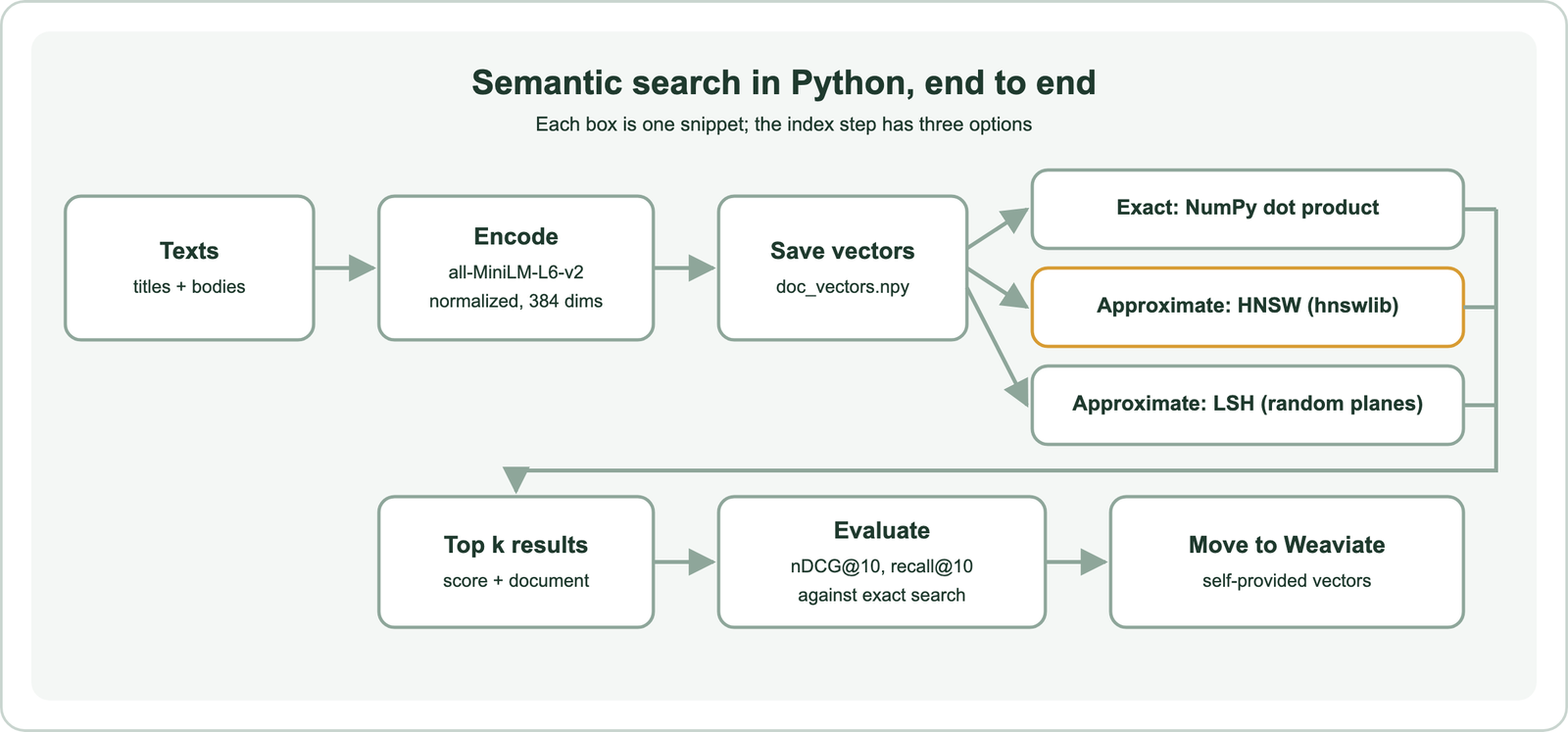
Every measured number in the tutorial comes from running the same code on BEIR SciFact, a public test set of 5,183 scientific abstracts and 300 queries with relevance labels. The environment was Python 3.9 with sentence-transformers 5.1.2, hnswlib, faiss-cpu 1.13.0 and NumPy 2.0.2 on one laptop CPU thread. Timings are for that machine only and are meant for comparing methods with each other. The first step is installing the libraries.
How do you install the Python libraries for semantic search?
You install the Python libraries for semantic search with pip: sentence-transformers for embeddings, plus hnswlib or faiss-cpu if you want an approximate index. The model weights download on first use and are cached locally.
pip install sentence-transformers hnswlib faiss-cpu scipySentence Transformers pulls in PyTorch and the Hugging Face transformers library. The example model, all-MiniLM-L6-v2, outputs 384 numbers per text and truncates input at 256 word pieces. That limit matters: a 2,000-word document is cut, and only its opening is embedded. Longer documents should be split into passages first, which is covered in semantic search over documents and PDFs.
One practical trap appeared during the test. Both PyTorch and faiss ship their own OpenMP runtime, and loading both in one macOS process crashed with a segmentation fault until OMP_NUM_THREADS was set to 1. Linux installs usually avoid the clash, but if a script dies silently after importing faiss, that variable is the first thing to try. Encoding speed then drops, since the model runs on one thread; the 5,183 abstracts took about four minutes.
The vectors themselves are small. At 384 dimensions in 32-bit floats, the whole SciFact corpus used 8.0 MB. A million documents would need about 1.5 GB, which still fits in memory on most servers. With the libraries installed, the first search is a few lines away.
How do you run a first semantic search with Sentence Transformers?
You run a first semantic search with Sentence Transformers by encoding the documents once, encoding the query, and calling util.semantic_search to get the most similar documents with their scores. The function does an exact cosine search and returns the top 10 by default.
from sentence_transformers import SentenceTransformer, util

docs = [
    "Reset your password from the account settings page.",
    "Refunds are issued to the original payment method within 5 days.",
    "Two-factor authentication adds a code sent to your phone.",
    "Export your invoices as CSV from the billing tab.",
    "Our office is closed on public holidays.",
    "You can change the email address linked to your account.",
]
model = SentenceTransformer("sentence-transformers/all-MiniLM-L6-v2")
doc_emb = model.encode_document(docs, normalize_embeddings=True, convert_to_tensor=True)

query = "I forgot my login credentials"
q_emb = model.encode_query(query, normalize_embeddings=True, convert_to_tensor=True)
for hit in util.semantic_search(q_emb, doc_emb, top_k=3)[0]:
    print(round(hit["score"], 3), docs[hit["corpus_id"]])
The run printed the password article first at 0.606, then the email article at 0.355 and two-factor authentication at 0.26. None of those documents contains “forgot”, “login” or “credentials”, which is the point of semantic search. The Sentence Transformers documentation recommends encode_query and encode_document for this kind of short-query, long-answer search, which it calls asymmetric. Models trained with separate query and document prompts use them; for all-MiniLM-L6-v2 they behave like plain encode.
Normalizing the embeddings makes every vector unit length, so a dot product equals cosine similarity. The documentation advises that combination for speed. util.semantic_search processes 100 queries at a time and splits the corpus into chunks of 500,000 by default. It is suitable, in the documentation’s words, for corpora up to about 1 million entries. On SciFact it scored 0.648 nDCG@10. The same search can be written without the helper.
How does exact semantic search work with NumPy?
Exact semantic search works with NumPy by multiplying the matrix of normalized document vectors by the normalized query vector and sorting the scores. Every document is scored, so the result is the true top k, with no approximation.
import numpy as np
from sentence_transformers import SentenceTransformer

docs = ["Reset your password from the account settings page.",
        "Refunds are issued to the original payment method within 5 days.",
        "Export your invoices as CSV from the billing tab."]
model = SentenceTransformer("sentence-transformers/all-MiniLM-L6-v2")
E = model.encode(docs, normalize_embeddings=True)          # shape (n, 384), float32
np.save("doc_vectors.npy", E)                             # embed once, reuse later

def search(query, k=2):
    q = model.encode(query, normalize_embeddings=True)
    scores = E @ q                                        # cosine, since both are unit length
    top = np.argsort(-scores)[:k]
    return [(float(scores[i]), docs[i]) for i in top]

print(search("how do I get my money back"))
The query “how do I get my money back” returned the refunds article at 0.492, with no shared words. Saving the matrix with np.save means the slow step, encoding, happens once; later runs load the file in milliseconds. On SciFact, the NumPy version and util.semantic_search returned identical top 10 lists for all 300 queries, and the matrix product took 0.30 ms per query.
Exact search cost grows in step with the corpus. Ten times more documents means roughly ten times more multiplications per query. For a help center or a product catalog of a few thousand items, that never matters. For millions of passages, or for many queries per second, an approximate index cuts the work by skipping most of the corpus. The approximate index that Weaviate uses by default is HNSW.
How do you add an HNSW index in Python with hnswlib?
You add an HNSW index in Python with hnswlib by creating an index with the cosine space and vector size, adding the document vectors, and setting the ef search parameter before querying. HNSW, a layered proximity graph, finds near neighbours by walking the graph instead of scoring every vector.
import hnswlib
import numpy as np

E = np.load("doc_vectors.npy")
index = hnswlib.Index(space="cosine", dim=E.shape[1])
index.init_index(max_elements=len(E), M=16, ef_construction=200)
index.add_items(E, np.arange(len(E)))
index.set_ef(50)                                          # higher ef: better recall, slower queries

labels, distances = index.knn_query(E[:1], k=2)           # cosine distance = 1 - similarity
print(labels, distances)
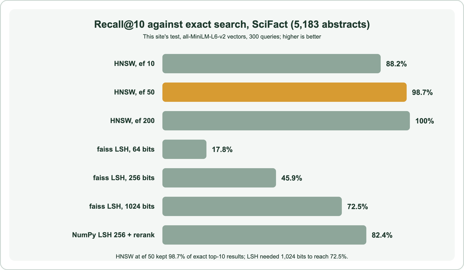
M sets how many links each node keeps, and ef_construction sets how hard the build searches for good links. At query time, ef sets how many candidates the search keeps in play. On SciFact, the index built in 0.3 seconds. With ef at 10, it returned 88.2 percent of the exact top 10, and nDCG@10 fell from 0.648 to 0.603. With ef at 50, recall reached 98.7 percent and nDCG@10 was 0.647. With ef at 200, the results matched exact search.
On a corpus this small, HNSW at ef 50 took 0.031 ms per query against 0.30 ms for NumPy, though both are effectively instant. The gap widens with corpus size. The trade-off between ef, recall and latency is covered in choosing a vector database for semantic search, since most databases expose the same knobs. An older family of approximate methods, LSH, behaves very differently.
How does locality sensitive hashing work for semantic search in Python?
Locality sensitive hashing works for semantic search in Python by projecting each vector onto random hyperplanes and keeping only the signs, so vectors pointing in similar directions get similar bit signatures. Search then compares short bit strings by Hamming distance instead of full vectors.
import numpy as np

E = np.load("doc_vectors.npy")
rng = np.random.default_rng(0)
planes = rng.standard_normal((E.shape[1], 256))           # 256 random hyperplanes
codes = np.packbits(E @ planes > 0, axis=1)               # one 256-bit signature per document

def lsh_search(q, k=10, shortlist=100):
    q_code = np.packbits(q @ planes > 0)
    hamming = np.unpackbits(codes ^ q_code, axis=1).sum(axis=1)
    shortlist = min(shortlist, len(E) - 1)
    cand = np.argpartition(hamming, shortlist)[:shortlist]
    return cand[np.argsort(-(E[cand] @ q))][:k]           # exact rerank of the shortlist

print(lsh_search(E[0], k=2))
The chance that two vectors fall on the same side of a random plane rises as the angle between them shrinks, which is why the signs preserve cosine neighbourhoods roughly. faiss offers the same idea as IndexLSH. On SciFact, faiss IndexLSH with 64 bits recovered only 17.8 percent of the exact top 10. With 256 bits it recovered 45.9 percent, and with 1,024 bits 72.5 percent. The NumPy version did better, at 82.4 percent, because it reranks a shortlist of 100 candidates with the real vectors.
The weak result is not a coding error; dense sentence embeddings cluster tightly, so many documents share most of their signature bits. LSH remains useful for near-duplicate detection and for very large, cheap first passes, but for semantic search over embeddings, HNSW gave far better recall here at similar speed. The next choice is how to measure distance at all.
Which distance should Python semantic search use: cosine, Euclidean or Minkowski?
Python semantic search should use the distance the embedding model was trained for, which for Sentence Transformers models is usually cosine similarity. On normalized vectors, Euclidean distance gives the same order as cosine, so the two are interchangeable.
Minkowski distance generalises the familiar metrics with a parameter p: p of 1 is Manhattan distance and p of 2 is Euclidean distance. SciPy computes it with cdist and metric set to minkowski. The snippet ranks one query against every document under three values of p.
import numpy as np
from scipy.spatial.distance import cdist

E = np.load("doc_vectors.npy")
q = E[:1]
for p in (1, 2, 3):
    d = cdist(q, E, metric="minkowski", p=p)[0]
    print(p, np.argsort(d))                              # smallest distance first
On SciFact, p of 2 returned exactly the cosine top 10 for every query, as the algebra predicts for unit vectors. Manhattan distance, p of 1, shared 84.4 percent of the cosine top 10 and scored 0.635 nDCG@10. Its score is lower than cosine’s 0.648. The p of 3 setting shared 89.3 percent and scored 0.649, a difference too small to matter on 300 queries. Nothing here justifies leaving cosine.
The deeper lesson is that the model, not the metric, decides quality. The ordering of Minkowski variants is close because they all measure the same embedding space. Changing the model, or how documents are split and indexed, moves results far more. Proving any of that requires an evaluation.
How do you evaluate a Python semantic search?
You evaluate a Python semantic search by running a set of real queries with known relevant documents and scoring the ranked results with a metric such as nDCG@10. For approximate indexes, you also compare their results with exact search using recall@10.
import math

def recall_at_k(approx, exact, k=10):
    return len(set(approx[:k]) & set(exact[:k])) / k

def ndcg_at_k(ranked_ids, relevant, k=10):
    gain = sum(1 / math.log2(i + 2) for i, d in enumerate(ranked_ids[:k]) if d in relevant)
    ideal = sum(1 / math.log2(i + 2) for i in range(min(k, len(relevant))))
    return gain / ideal

print(recall_at_k([3, 1, 7], [1, 3, 4], k=3), round(ndcg_at_k([3, 1, 7], {1, 4}, k=3), 3))
The example prints 0.667 and 0.387. Two of three exact results were found, and the one relevant hit sat in second place with a second relevant document missing. Recall against exact search isolates the index: it says nothing about whether the documents are relevant, only whether the shortcut lost any. nDCG against labels measures what users see.
| Option | Recall@10 vs exact | nDCG@10 | ms per query |
|---|---|---|---|
| NumPy dot product (exact) | 100% | 0.648 | 0.30 |
| hnswlib, ef 50 | 98.7% | 0.647 | 0.031 |
| NumPy LSH, 256 bits, rerank 100 | 82.4% | 0.641 | 0.55 |
| faiss IndexLSH, 1,024 bits | 72.5% | 0.612 | 0.035 |
The table shows that a lossy index costs relevance roughly in proportion to the neighbours it drops. The same evaluation harness should guard any change of model or chunking. How to evaluate semantic search covers building a query set. Once quality is proven, the script usually needs a real database.
How do you move a Python semantic search into Weaviate?
You move a Python semantic search into Weaviate by creating a collection with self-provided vectors, importing each document with its existing embedding, and querying with near_vector or hybrid. The embedding model stays in your Python code, so results match the script’s.
import numpy as np
import weaviate
from weaviate.classes.config import Configure, Property, DataType
from weaviate.classes.query import MetadataQuery
from sentence_transformers import SentenceTransformer

docs = ["Reset your password from the account settings page.",
        "Refunds are issued to the original payment method within 5 days.",
        "Export your invoices as CSV from the billing tab."]
model = SentenceTransformer("sentence-transformers/all-MiniLM-L6-v2")
E = np.load("doc_vectors.npy")

client = weaviate.connect_to_embedded()  # weaviate.connect_to_local() for a Docker instance
try:
    client.collections.delete("HelpArticle")
    articles = client.collections.create(
        name="HelpArticle",
        vector_config=Configure.Vectors.self_provided(),
        properties=[Property(name="body", data_type=DataType.TEXT)],
    )
    with articles.batch.fixed_size(batch_size=100) as batch:
        for text, vec in zip(docs, E):
            batch.add_object(properties={"body": text}, vector=vec.tolist())

    q = model.encode("how do I get my money back", normalize_embeddings=True)
    res = articles.query.near_vector(near_vector=q.tolist(), limit=2,
                                     return_metadata=MetadataQuery(distance=True))
    for o in res.objects:
        print(round(o.metadata.distance, 3), o.properties["body"])
    res = articles.query.hybrid(query="money back", vector=q.tolist(), alpha=0.5, limit=2)
    for o in res.objects:
        print("hybrid", o.properties["body"])
finally:
    client.close()
The run used Weaviate Python client 4.18.3 with an embedded Weaviate 1.30.5 server. It returned the refunds article at a cosine distance of 0.508, which is 1 minus the 0.492 similarity from the NumPy script. Weaviate’s documentation describes this bring-your-own-vectors pattern. With a self-provided configuration, every import and every vector query must carry a vector, because Weaviate cannot embed text on its own. The hybrid query adds BM25 keyword matching at no extra modelling cost.
The database adds what the script lacks: persistence, filters, an HNSW index managed for you, and keyword search. Semantic search with Weaviate covers its built-in vectorizers. The remaining question is when to make that move.
When does a Python script stop being enough for semantic search?
A Python script stops being enough for semantic search when the corpus changes often, needs metadata filters or keyword matching, or serves many users at once. Until then, a NumPy array and a saved file are simpler than any database.
The script keeps everything in one process, so every update means re-encoding and re-saving, and every server holds its own copy. Databases solve those problems in different ways. Weaviate and the other dedicated engines compared in choosing a vector database each have a Python tutorial: Weaviate, Qdrant, Milvus, Pinecone, Chroma and Redis. Teams already running a search engine or Postgres can add vectors there, in Elasticsearch, OpenSearch or Postgres with pgvector.
Frameworks offer a shortcut over the plumbing. LangChain and LlamaIndex wrap loading, splitting, embedding and storing in a few calls, at the cost of hiding the steps measured here. Whatever the destination, keep the saved vectors and the model name together. Switching the model later means re-embedding everything, and migrating to a new vector database is much easier with that file in hand.
A sensible path has three stages: prove quality with NumPy and an evaluation set, add HNSW when speed demands it, and move to a database when updates, filters or traffic demand it.
Semantic search in Python comes down to an embedding model, a matrix of normalized vectors and a way to find the nearest ones. Sentence Transformers handles the first, NumPy handles exact search for most small and medium corpora, and hnswlib adds an HNSW index that matched exact results at ef 50 in this site’s SciFact test. Random-hyperplane LSH was the weak option, and Minkowski or Euclidean distance added nothing over cosine on unit vectors. Measure with nDCG@10 and recall@10 before and after every change. When the data needs updates, filters or keyword matching, move the same vectors into Weaviate or another database without re-embedding.