Home / Filtering / Filter Selectivity and Its Effect on Search Speed

Filter Selectivity and Its Effect on Search Speed

Filter selectivity is the share of a collection that passes a filter, and it decides which execution plan makes a filtered vector search fastest. When very few objects match, the quickest plan is to compute distances for just those objects, a flat search. When most objects match, a normal graph search that checks the filter as it goes works well. In between, the graph search must skip non-matching objects without losing its way, which is what methods such as ACORN address. Selectivity also decides how many candidates post-filtering must fetch. With 1 percent of objects passing, keeping 10 results takes about 1,000 candidates. In Weaviate, the default flat-search cutoff is 40,000 matching objects, and ACORN is the default filter strategy from version 1.34. Correlation between the filter and the query shifts the picture further.

What is filter selectivity?

Filter selectivity is the proportion of objects in a collection that satisfy a filter condition, such as price under 200 or language equal to German. It is a property of the filter and the data together, not of the filter alone.

A filter that 2 of 1,000 products pass has a pass rate of 0.2 percent. One that 900 of them pass has a pass rate of 90 percent. The same filter can have very different selectivity in two collections, or in the same collection as data changes. A filter on “in stock” may pass most products in one season and few in another.

The vocabulary is confusing because sources use the word both ways. Database texts often call a filter “highly selective” when it passes few rows. Some vector search writing, including Weaviate’s blog on ACORN, uses “selectivity rate” for the share of objects that pass. Here the terms “pass rate” and “few objects match” are used to avoid the ambiguity. Filters themselves are introduced in metadata filtering.

How do you measure the selectivity of a filter?

You measure the selectivity of a filter by counting how many objects pass it and dividing by the total object count. Most databases can count matches cheaply from their inverted indexes, without running any vector search.

from weaviate.classes.query import Filter

products = client.collections.use("Product")
f = Filter.by_property("price").less_than(20)
matches = products.aggregate.over_all(filters=f, total_count=True).total_count
total = products.aggregate.over_all(total_count=True).total_count
print(matches, total, matches / total)

Run this for the filters your application actually sends, not only for single fields. Combined filters multiply: if 10 percent of products are shoes and 10 percent are on sale, and the two are independent, about 1 percent are shoes on sale. Real fields are rarely independent, so measure the combinations rather than estimating them.

Log pass rates alongside query latency in production. A latency spike that only affects some queries often traces back to a small set of filters with very low or very high pass rates. That link is hard to see without the counts. Production measurement more broadly is covered in search latency.

Which execution plans does selectivity decide between?

Selectivity decides between three broad plans: a flat scan of the matching objects, a graph search that skips non-matching objects, and a normal graph search that checks the filter as results are added. Each is fastest in a different range of pass rates.

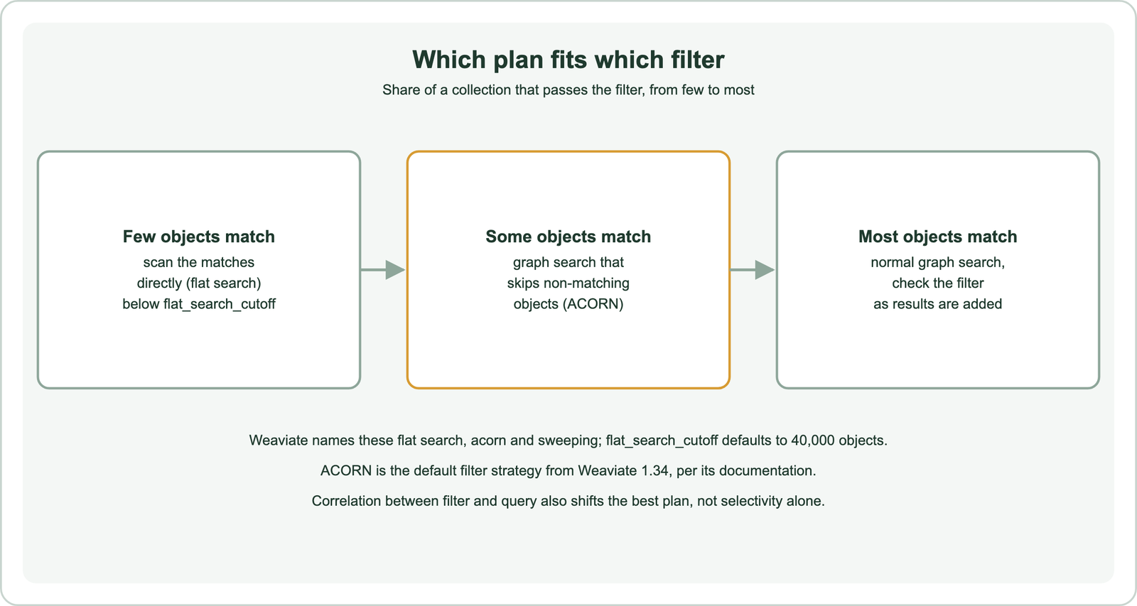
A flat scan computes the distance from the query to every matching object and keeps the closest. Its cost grows with the number of matches, so it is cheap when matches are few and wasteful when they are many. A graph search through an index such as HNSW is cheap when it can move freely towards the query, but a strict filter blocks many of its steps.

The best plan therefore flips as the pass rate changes. Systems that pick one plan for every query tend to be fast on some filters and slow on others. The broader comparison of filtering orders is in pre-filtering vs post-filtering, and the graph-side methods in filtered ANN search.

How should a search run when few objects match?

When few objects match, the search should skip the vector index and compute distances for the matching objects directly, because a flat scan of a small set is both fast and exact. Graph traversal under a very strict filter visits many nodes it cannot return.

Weaviate’s documentation explains the reasoning. As a filter becomes more restrictive, an HNSW traversal becomes close to exhaustive, so its cost approaches brute force over the whole collection. Brute force over only the matching subset is far cheaper. Weaviate therefore switches to flat search when fewer objects match than flat_search_cutoff, 40,000 by default, configurable per collection.

A flat scan also gives exact results, with no recall loss from approximation. For filters such as one customer’s documents or one narrow category, that makes it the right plan, not a fallback. Per-tenant collections take the same idea further by keeping each tenant’s data in its own index, as described in multi-tenant semantic search.

How should a search run when most objects match?

When most objects match, the search can traverse the graph almost as if there were no filter, checking each candidate against the filter before adding it to the results. Few candidates are rejected, so little work is wasted.

Weaviate calls this strategy sweeping. The search moves through the HNSW graph as usual and keeps the filter’s allow list as context. Nodes that fail the filter can still be traversed, so the graph stays connected, but they are not added to the result set. The search stops when it has enough passing results and further candidates no longer improve them.

Weaviate’s ACORN blog reports internal tests in which sweeping performed better at a 50 percent pass rate and ACORN performed better at 20 percent. That matches the intuition: sweeping wastes distance calculations on rejected objects, and the waste grows as the pass rate falls. The same blog notes that Weaviate’s ACORN implementation switches back to sweeping when it detects a filter that most objects pass.

Why are mid-range and low pass rates hardest for graph search?

Mid-range and low pass rates are hardest for graph search because too many objects fail to ignore, yet too many pass for a cheap flat scan. Skipping failing nodes outright risks disconnecting the graph.

HNSW finds neighbours by hopping from node to node towards the query. If the search refuses to step on nodes that fail the filter, some regions become unreachable, and recall drops. If it steps on them but discards them, it spends distance calculations on objects it can never return. Either way, a strict filter that is not strict enough for a flat scan makes the graph search slower or less accurate.

ACORN, from a 2024 paper by Patel and colleagues, addresses this by expanding the neighbourhood two hops at a time. It looks past failing neighbours to their passing neighbours, keeping the filtered subgraph connected without computing distances for failing objects. Weaviate’s own implementation, inspired by the paper, also seeds extra entry points that match the filter. It needs no re-indexing.

How does selectivity affect post-filtering?

Selectivity sets how many candidates post-filtering must fetch: to keep k results, it needs about k divided by the pass rate. Post-filtering runs an unfiltered vector search first and removes failing results afterwards.

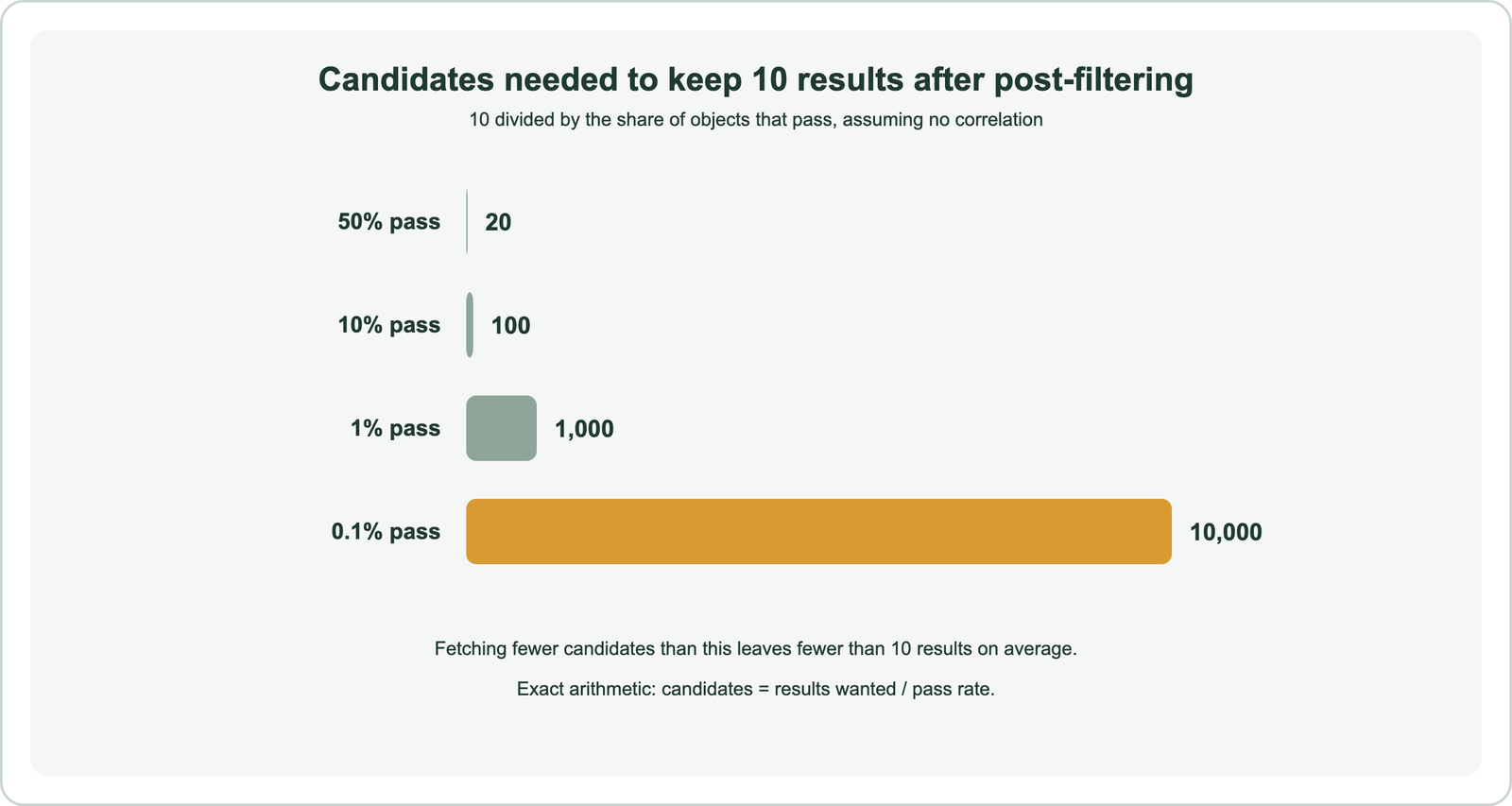
At a 50 percent pass rate, 20 candidates leave about 10 results. At 1 percent, 1,000 candidates are needed, and at 0.1 percent, 10,000. These numbers assume the filter is unrelated to the query. Fetch fewer, and the search returns short or empty result lists, a common bug in systems that post-filter with a fixed candidate count.

Weaviate avoids this problem by building an allow list from its inverted index before the vector search, then searching only for allowed objects. Its documentation describes this as pre-filtering that does not require a brute-force search. Engines that only post-filter must estimate the pass rate and oversample, which is fragile when selectivity varies by query.

How does correlation between filter and query change selectivity?

Correlation changes the effective selectivity near the query: a filter can pass 50 percent of the whole collection yet almost none of the objects closest to the query. The local pass rate, not the global one, decides how hard the search is.

Weaviate’s ACORN blog gives an example. Searching an online ring shop for diamond rings with a high price filter is positively correlated: most nearby objects are expensive and pass. The same search with a very low price filter is negatively correlated: the nearest objects are expensive and fail, so the search must travel far through the graph to find cheap matches.

Negatively correlated filters are where ACORN helps most, according to Weaviate’s documentation. Positively correlated filters are easy for sweeping because filtered and unfiltered results are similar. A global pass rate cannot reveal which case a query is in, so test both kinds of filter on your own data. Hybrid queries add a keyword side with its own behaviour, covered in hybrid search on distributed databases.

How does data layout affect filter speed?

Data layout affects filter speed because a filter that matches contiguous blocks of stored data can skip everything else, while one that matches scattered objects cannot. Clustering or sorting data by commonly filtered fields creates that contiguity.

When storage is sorted by a list of clustering fields, rows are ordered by the first field, then by the second within each value of the first, and so on. A filter on the first field selects a few long runs and skips the rest. A filter on a later field matches short runs spread across every value of the earlier fields, so less can be skipped. That is why filters on fields listed earlier in a clustering key generally gain more from clustering.

Inverted indexes and bitmaps make the matching side fast regardless of layout. Weaviate’s allow list is a list of 64-bit identifiers built from its inverted index, which stays efficient as it grows. Compact bitmap structures for allow lists are covered in bitmap filters, and filter-driven navigation in faceted semantic search.

How do you tune filtered search for selectivity in Weaviate?

In Weaviate you tune filtered search for selectivity with two HNSW settings per collection: the filter strategy and the flat-search cutoff. Defaults suit most collections; change them only after measuring.

from weaviate.classes.config import Configure, VectorFilterStrategy

vector_index_config=Configure.VectorIndex.hnsw(
    filter_strategy=VectorFilterStrategy.ACORN,  # or SWEEPING
    flat_search_cutoff=40000,
)

Raise the cutoff if filters that match somewhat more than 40,000 objects are slow and exact results would be welcome. Lower it if flat scans of large match sets dominate latency. Compare ACORN with sweeping on a sample of real queries with their real filters, measuring recall and latency together. Weaviate’s documentation also lists a third strategy, pathseer, worth including in that comparison where the installed version supports it.

Selectivity also interacts with security filters. Permission filters often pass a small, user-specific fraction of the collection, which is exactly the hard range, as covered in permission-aware search. Choosing a database for this workload is covered in vector databases with metadata filtering, and when to filter versus search in searching vs filtering.

Filter selectivity is the share of a collection that passes a filter, and it decides the fastest plan for a filtered vector search. Few matches favour a flat scan, which Weaviate uses under 40,000 matching objects by default. Most matches favour sweeping, a graph search that checks the filter as it goes. The hard middle, and filters negatively correlated with the query, favour ACORN, Weaviate’s default strategy from version 1.34. Post-filtering needs about k divided by the pass rate in candidates, 1,000 for 10 results at 1 percent. Measure pass rates for real filters, test strategies on real queries, and watch local correlation, not just the global rate.