Home / Filtering / Bitmap Filters in Search Engines

Bitmap Filters in Search Engines

A bitmap filter represents the objects that match a condition as a sequence of bits, one bit per object. A search engine can then combine conditions with fast bitwise operations instead of comparing values one by one. Each indexed value, such as “color = red”, gets its own bitmap in which a 1 marks every object that has the value. A query with several conditions becomes an AND, OR or NOT over those bitmaps, and the result is the list of objects that pass. Compressed formats such as Roaring bitmaps keep the bitmaps small even when collections hold millions of objects. Vector databases use the result as an allow list that limits which objects the vector search may return. Weaviate builds a Roaring bitmap index for every filterable property by default, and its 1.18 release notes report filtered queries that fell from 3 to 4 seconds to 3 to 4 milliseconds in internal testing.

What is a bitmap filter?

A bitmap filter is a filter evaluated with bitmaps, arrays of bits in which position n is 1 when object n matches a condition and 0 when it does not. The bitmap is a compact way to store a set of object IDs.

Take a collection of products. The bitmap for “color = red” has a 1 at the position of every red product. The bitmap for “in stock = true” has a 1 at every product in stock. To find red products in stock, the engine does not inspect each product. It takes the two bitmaps and computes their bitwise AND, which leaves a 1 only where both conditions hold.

The idea is old and well proven. Relational databases and data warehouses have offered bitmap indexes for decades, mainly for columns with few distinct values, such as status, region or category. Search engines use the same structure for filters and facets, and vector databases use it to restrict a similarity search to objects that meet structured conditions.

Filters of this kind are one part of metadata filtering. The bitmap is the data structure that makes those filters cheap enough to run on every query.

How does a bitmap index work?

A bitmap index stores one bitmap for each distinct value of a property and answers a filter by reading the bitmaps for the requested values and combining them with bitwise operations. Building the index happens at import time, so queries only read and combine.

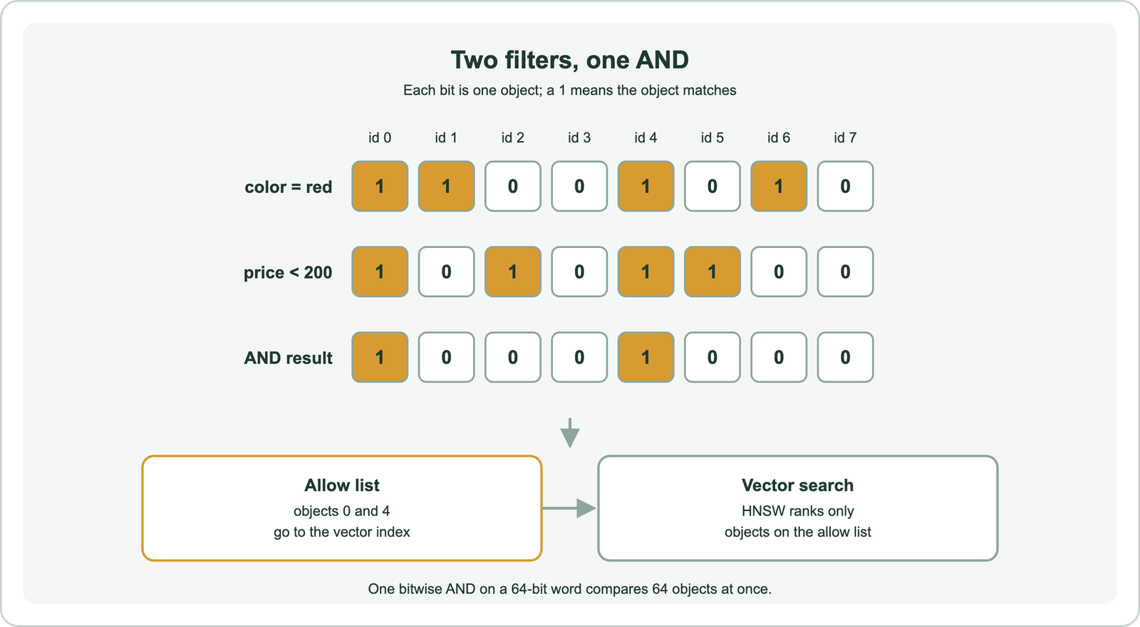
The operations map directly to filter logic. AND gives the intersection of two conditions, OR gives their union, and NOT gives the complement. A filter such as “red or blue, and under 200, and not discontinued” becomes a short sequence of those operations, whatever the size of the collection.

The speed comes from the hardware. A processor computes a bitwise AND on a 64-bit word in one instruction, so each instruction compares 64 objects at once. Modern processors also offer wider vector instructions. Counting the 1 bits in the result, which gives the number of matches, is also a single instruction per word on most processors.

The cost is space. An uncompressed bitmap needs one bit per object for every value, so a collection of 1,000,000 objects needs 1,000,000 bits, or 125,000 bytes, per value. A property with thousands of distinct values, most of them rare, would waste most of that space on zeros. Compression solves this problem.

How do Roaring bitmaps compress filters?

Roaring bitmaps compress a set of IDs by splitting the ID space into chunks of 65,536 values and storing each chunk in whichever container is smallest for its contents. The format was introduced by Chambi, Lemire, Kaser and Godin in 2016 and is now widely used.

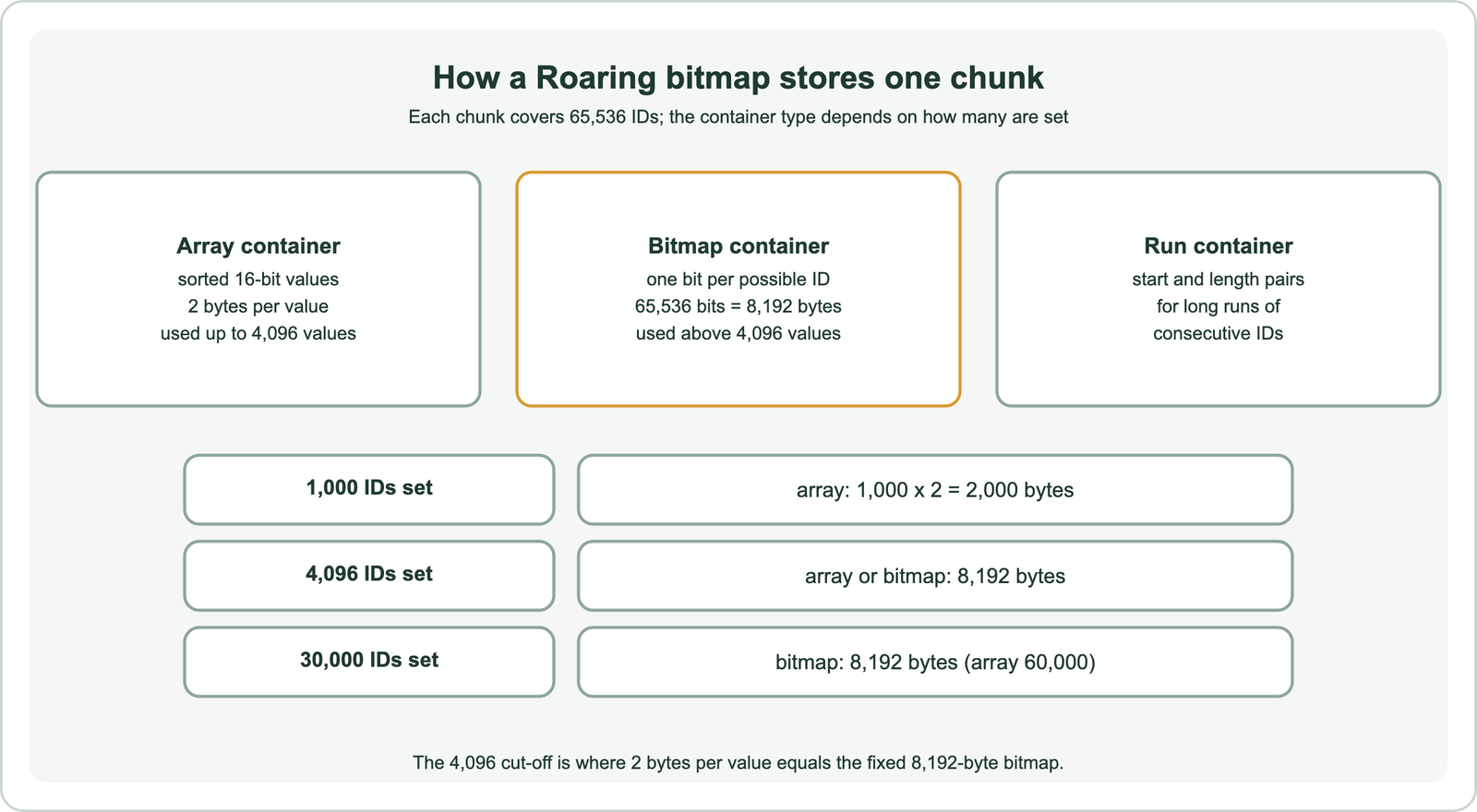
The high 16 bits of each ID choose the chunk, and the low 16 bits are stored in the chunk’s container. A sparse chunk uses an array container, a sorted list of 16-bit values at 2 bytes each. A dense chunk uses a bitmap container of 65,536 bits, which is 8,192 bytes. The switch happens at 4,096 values, because 4,096 values at 2 bytes each also take 8,192 bytes. A later version added run containers for long stretches of consecutive IDs.

Operations stay fast because each pair of containers has its own algorithm. Intersecting two arrays merges sorted lists, intersecting two bitmaps uses word-wide AND, and intersecting an array with a bitmap checks each array value against the bitmap. Empty chunks are skipped entirely.

Weaviate adopted Roaring bitmaps in version 1.18 for its inverted index and extended them to text properties in 1.19. Its release notes say the change made some filtered searches up to 1,000 times faster, with queries that took 3 to 4 seconds finishing in 3 to 4 milliseconds in internal testing. Weaviate maintains its own Roaring bitmap library.

How do bitmaps handle range filters?

Bitmaps handle range filters either by combining the bitmaps of every value in the range, or by using a bit-sliced layout that answers a range with a fixed number of operations. The second approach is far cheaper for numbers and dates with many distinct values.

A plain bitmap index answers “price under 200” by reading the bitmap for every price under 200 and computing their OR. With thousands of distinct prices, that means thousands of bitmaps per query. Weaviate’s FAQ describes a range lookup as a set of range reads over the value rows, which is efficient but grows with the number of values covered.

A bit-sliced index stores numbers differently. It keeps one bitmap per bit position of the value, so a 64-bit number needs at most 64 bitmaps no matter how many distinct values exist. A comparison walks those bit positions in order and combines them, so its cost depends on the bit width, not on the size of the range. Weaviate’s indexRangeFilters, added in version 1.26, uses this idea, implemented as Roaring bitmap slices.

Weaviate’s documentation sets the rules. The range index applies to int, number and date properties, not to arrays of them, and it limits values to those that fit in 64-bit integers. It is off by default and can only be set on new properties. When both indexes exist, Weaviate uses the range index for greater-than and less-than comparisons and the filterable index for equal and not-equal.

How do vector databases use bitmap filters?

Vector databases use bitmap filters to build an allow list of matching objects before the vector search, then let the vector index return only objects on that list. This is pre-filtering, and it guarantees that every result meets the filter.

Weaviate describes the process in two steps. The inverted index produces an allow list of matching object IDs. The HNSW index then searches as usual, moving along graph edges, but adds an ID to the result set only if it is on the allow list. Non-matching objects can still be visited as stepping stones through the graph. The trade-offs against filtering after the search are covered in pre-filtering vs post-filtering.

The size of the allow list shapes the cost. Weaviate’s FAQ explains that a loose filter costs little more than an unfiltered search, while a very restrictive filter can force the search to visit many non-matching nodes. For small allow lists, Weaviate skips the graph and compares vectors directly, controlled by the flatSearchCutOff parameter. The effect of match rates is the subject of filter selectivity.

Graph strategies handle the hard middle. Weaviate’s ACORN strategy, the default since version 1.34, ignores non-matching objects in distance calculations, uses two-hop expansion to reach matching regions faster and seeds extra entry points that pass the filter. The wider set of techniques is described in filtered ANN search.

How do you configure bitmap filtering in Weaviate?

You configure bitmap filtering in Weaviate per property, keeping index_filterable on for equality filters and turning on index_range_filters for numbers and dates queried by range. Null-state indexing is a collection setting.

from weaviate.classes.config import (Configure, Property, DataType,
                                     Tokenization, VectorFilterStrategy)
from weaviate.classes.query import Filter

products = client.collections.create(
    "Product",
    vector_config=Configure.Vectors.self_provided(
        vector_index_config=Configure.VectorIndex.hnsw(
            filter_strategy=VectorFilterStrategy.ACORN)),
    inverted_index_config=Configure.inverted_index(index_null_state=True),
    properties=[
        Property(name="name", data_type=DataType.TEXT),
        Property(name="color", data_type=DataType.TEXT,
                 tokenization=Tokenization.FIELD, index_searchable=False),
        Property(name="price", data_type=DataType.NUMBER, index_range_filters=True),
        Property(name="discount", data_type=DataType.NUMBER),
    ],
)

f = Filter.by_property("color").equal("red") & Filter.by_property("price").less_than(200)
res = products.query.near_vector(query_vector, filters=f, limit=10)
count = products.aggregate.over_all(filters=f, total_count=True).total_count

The color property keeps its filterable bitmap index but skips the searchable BM25 index, since nobody searches colors by keyword. The price property gets the range index for the less-than comparison. The aggregate call counts matches with the same filter, which helps estimate selectivity. The snippet was run on Embedded Weaviate 1.30.5 as an API check only.

Weaviate’s rule of thumb is simple: if you will never query by a property, you can turn its index off. Disabling unused indexes speeds up imports and saves disk. More on choosing which properties to index is in vector databases with metadata filtering.

What is a null bitmap?

A null bitmap is a bitmap that records which values are missing, either per row inside a database record or per property across a collection. The term covers two related uses.

In relational databases, a null bitmap often sits in the row header. PostgreSQL, for example, adds a null bitmap to a row only when the row contains nulls, with one bit per column. The database then skips storing those columns at all, which saves space and tells the reader which fields are absent.

In search engines, a null-state index works like any other bitmap filter: one bitmap marks the objects where a property is missing. Weaviate builds this index when index_null_state is enabled in the collection’s inverted index settings, and the is_none filter then finds objects with or without a value. In the snippet, filtering on a missing discount returns only the product that has none.

When are bitmap filters not enough?

Bitmap filters are not enough when the main cost lies elsewhere, such as in a vector search constrained by a very restrictive filter, or in properties that change constantly. The bitmap step itself is rarely the bottleneck.

A fast allow list does not make the following vector search fast. If only a tiny share of objects match and they sit far from the query in vector space, the graph search still has to work hard. That is why flat search cut-offs and strategies such as ACORN exist. Splitting data by tenant, as in multi-tenant semantic search, can remove the most common restrictive filter altogether.

Write-heavy properties carry an import cost, because every change updates the bitmaps. Free text used only for search does not need a filterable index. Some conditions belong in search rather than in filters, a distinction covered in searching vs filtering. Bitmaps also power facet counts, as in faceted semantic search, and access rules, as in permission-aware search.

A bitmap filter stores the objects that match a condition as bits, one per object, so conditions combine with bitwise AND, OR and NOT at 64 objects per instruction. Roaring bitmaps keep the index small by storing each chunk of 65,536 IDs as an array, a bitmap or runs, switching at 4,096 values. Weaviate uses Roaring bitmaps for its filterable index and Roaring bitmap slices for range filters on numbers and dates. The result becomes the allow list that the HNSW index respects during vector search. Keep filterable indexes on properties you filter by, add range indexes where you compare numbers, and turn indexes off where you never query.