Home / How it works / Semantic Search Architecture: A Reference Diagram
ExplainerSemantic Search Architecture: A Reference Diagram
A semantic search architecture has two separate paths: an indexing path that turns content into embeddings and stores them, and a query path that embeds each search and retrieves the closest matches. The indexing path runs ahead of time: parse sources, split them into chunks, embed each chunk, and write vectors, text, and metadata to a vector database. The query path runs on every search: understand the query, embed it with the same model, retrieve candidates with vector and keyword search under filters, rerank, and return results or a generated answer. On one laptop CPU, embedding a query took about 2 ms in this site’s test, while reranking 20 results took 42.5 ms. That is why reranking, not vector search, usually sets the latency budget.
Semantic search architecture in four facts
- Indexing and querying are separate paths that must use the same embedding model.
- A Weaviate shard holds three stores together: objects, an inverted index, and a vector index.
- In this site’s timing test, a cross-encoder rerank of 20 results took 42.5 ms; exact search over 100,000 vectors took 2.3 ms.
- Sharding scales data size and import speed; replication scales query throughput and availability.
What is semantic search architecture?
Semantic search architecture is the set of components and data flows that let a system find content by meaning. Its parts are an embedding model, a store with a vector index, and the pipelines that feed and query it. It is the engineering behind what users experience as “search that understands”.
The core idea fits in one sentence. Content and queries are both converted into vectors by the same embedding model, and search becomes finding the stored vectors closest to the query vector. Everything else in the architecture exists to make that reliable at scale: getting clean text in, keeping indexes current, combining meaning with exact matches, and ranking the best results first.
Most production systems share the same skeleton, whatever the vendor. DataHub’s published design, for example, adds semantic search beside its existing keyword index rather than replacing it, with embeddings generated at ingestion and a k-NN index for queries. What is semantic search covers the concept; the architecture is about the parts and how they connect.
What does a reference architecture diagram show?
A reference architecture diagram shows the indexing path and the query path as two separate flows that meet at the shared indexes. Drawing them apart makes clear which work happens once per document and which happens once per search.
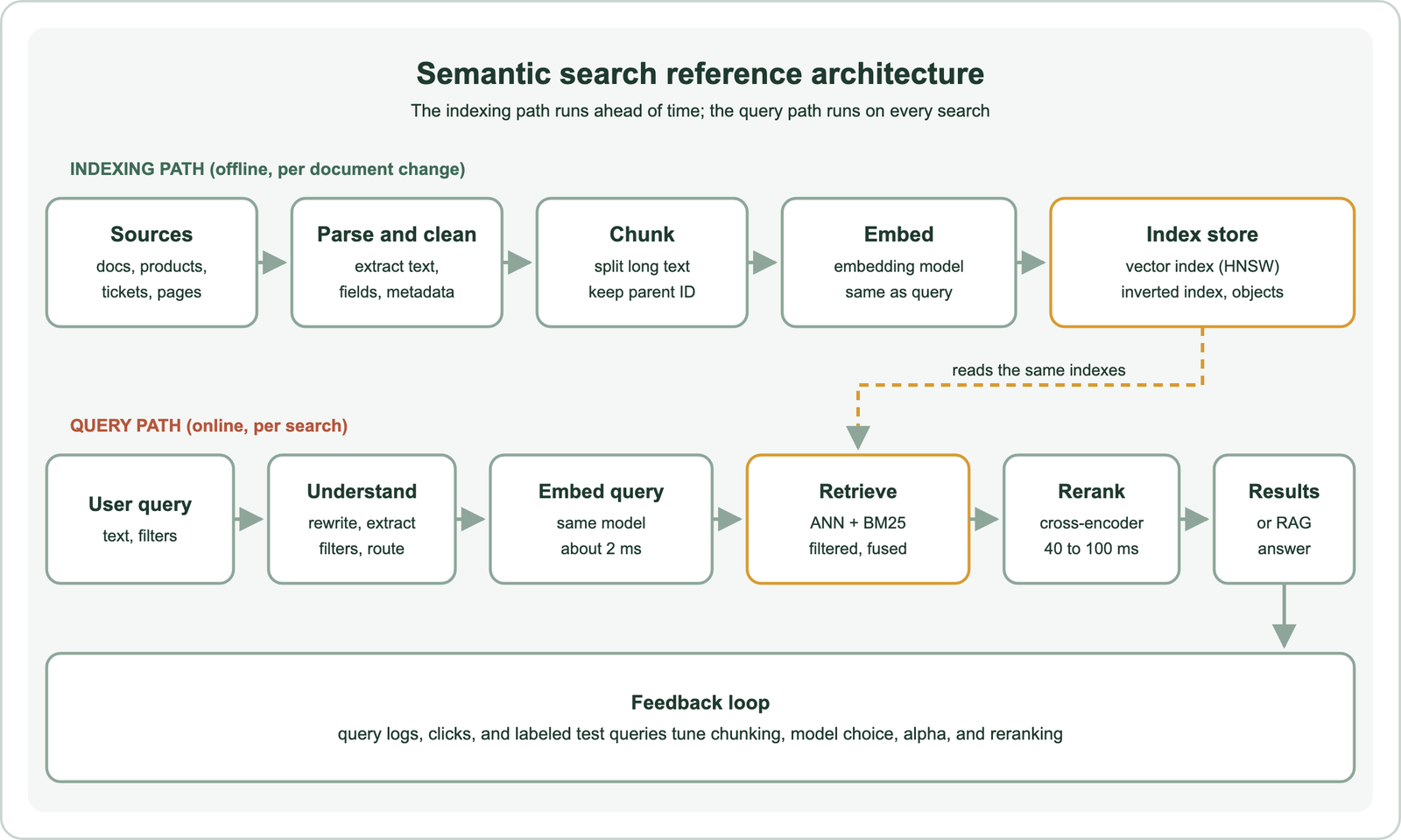
The two paths have different performance goals. Indexing cares about throughput: how many documents per second can be parsed, embedded, and written. Querying cares about latency: how many milliseconds a user waits. Keeping them separate lets each scale on its own, for example by batching embeddings on a GPU at ingestion while queries run on CPU nodes.
A third loop sits around both. Query logs, clicks, and a labeled test set tell you whether chunk sizes, the embedding model, the keyword weight, and the reranker are working. Without that loop, an architecture can run smoothly and still return the wrong results.
How does the indexing path work?
The indexing path works by extracting text and metadata from sources, splitting long text into chunks, embedding each chunk, and writing the vectors with their text and metadata into the store. It runs at first load and again whenever content changes.
- Extract: pull text and fields from documents, product feeds, tickets, or web pages, including OCR or transcription where needed.
- Clean and enrich: remove boilerplate, normalize text, and attach metadata such as source, date, author, and access rights.
- Chunk: split long documents into passages that fit the model’s input limit, keeping a parent ID for each chunk.
- Embed: run each chunk through the embedding model.
- Write: store the object, its vector, and its metadata, which updates the vector and inverted indexes.
Weaviate Academy describes the write step from the database side. An incoming object passes through the API, gets vectorized if a vectorizer is configured, is stored in the object store, and then updates both the vector index and the inverted indexes. Weaviate can call the embedding model itself through a vectorizer module, or accept vectors you computed elsewhere.
Embedding is usually the slow part of indexing. In our timing test, the open all-MiniLM-L6-v2 model embedded about 614 passages of 40 words per second on a laptop CPU, at batch size 64. At that rate, one million passages would take roughly 27 minutes. Larger models, longer chunks, or a paid API change that figure, so measure it before planning a reindex. Chunking for semantic search covers the chunk step.
How does the query path work?
The query path works by interpreting the query, embedding it with the indexing model, retrieving candidates from the vector and keyword indexes, fusing and reranking them, and returning results or an answer. Each step is optional except embedding and retrieval.
Weaviate’s integration with Cohere shows the minimal version: receive the query, send it to the model to vectorize, search the vector index with the returned vector, and return matched objects. Production systems usually add steps on either side. Before retrieval, a query-understanding step can rewrite the query, extract filters such as a price limit, or route code-like queries to exact lookup.
Retrieval itself is often hybrid. A vector search finds meaning matches, a BM25 search finds exact terms, and a fusion step merges the two lists. Filters on metadata, such as date or access rights, apply during retrieval. After retrieval, a reranker can reorder the top candidates, and a language model can turn them into an answer. How hybrid search works covers the fusion step.
Where does query time go?
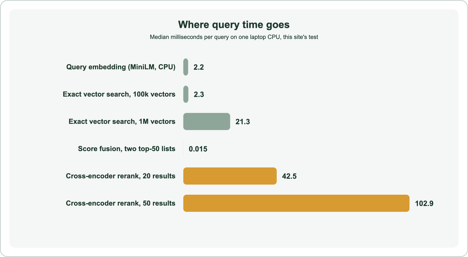
Query time goes mostly to reranking and to the embedding model when one is used, while vector retrieval over an index and score fusion take little time. We timed each stage on one laptop CPU to see the budget.
| Stage | Setup | Median time |
|---|---|---|
| Query embedding | all-MiniLM-L6-v2, one query | 2.2 ms |
| Exact vector search | 100,000 normalized 384-dim vectors, top 50 | 2.3 ms |
| Exact vector search | 1,000,000 vectors, top 50 | 21.3 ms |
| Score fusion | two top-50 lists, relative score | 0.015 ms |
| Cross-encoder rerank | ms-marco-MiniLM-L-6-v2, 20 pairs | 42.5 ms |
| Cross-encoder rerank | 50 pairs | 102.9 ms |
Exact search scales linearly, so 1 million vectors took about ten times as long as 100,000. An approximate index such as HNSW avoids that growth; Weaviate’s documentation cites sub-50 ms queries for 20 nearest neighbors on datasets of 1 to 100 million objects. Reranking scales with the number of candidates, so 50 pairs took about 2.4 times as long as 20.
The practical rule follows from the numbers. Spend the latency budget on reranking only as many candidates as you need, and run the reranker on a GPU if the volume justifies it. A hosted embedding API adds a network round trip, often more than the local model’s 2 ms. The recall versus latency trade-off covers index tuning.
How does Weaviate store the indexes?
Weaviate stores each collection as one or more shards, and each shard holds an object store, an inverted index, and a vector index side by side. That layout lets one shard answer a filtered, hybrid query on its own.
The object store and inverted index use a log-structured merge tree, or LSM tree. Writes land in memory first and are flushed to sorted disk segments, which are merged in the background. Bloom filters skip segments that cannot hold a requested object. Weaviate’s documentation notes this keeps ingestion fast as data grows.
The vector index sits next to these stores rather than inside them, and the default is a custom HNSW implementation. HNSW graphs cannot be merged efficiently, so Weaviate keeps each shard’s vector index as large as possible. It persists the graph with a write-ahead log and snapshots. Weaviate Academy lists four vector index types: hnsw, flat, dynamic, and the disk-based hfresh.
Keeping the stores together pays off at query time. Weaviate applies filters before the vector search, using the inverted index to build an allow list, so a filtered query still returns the requested number of results. Its documentation contrasts this with post-filtering, where the final count is unpredictable. Pre-filtering versus post-filtering explains the difference.
How does a semantic search architecture scale?
A semantic search architecture scales by sharding data across nodes to handle size and import speed, and by replicating shards to handle query throughput and availability. The two solve different problems and are often combined.
| Goal | Sharding | Replication |
|---|---|---|
| Dataset larger than one node | Yes | No |
| Faster imports | Yes | No |
| Higher query throughput | Partial | Yes, near linear |
| High availability and rolling upgrades | No | Yes |
Weaviate places objects on shards with a 64-bit Murmur-3 hash of each object’s UUID. Resharding is costly because of the HNSW structure, so the shard count is set when a collection is created. Weaviate’s documentation recommends several shards even on a single node, to use multiple CPUs and speed up imports.
Memory usually forces the first scaling decision, because HNSW graphs live in memory. Vector quantization compresses vectors by about 75 to 97 percent, depending on the method, and disk-based indexes reduce the need to shard for memory alone. For many separate customers with the same schema, multi-tenancy gives each tenant its own shard. Scaling semantic search goes further.
Should the embedding model run inside or outside the database?
The embedding model should usually run as a separate service from the database, either through a vectorizer module that calls it or in your own pipeline, so each can scale on its own hardware. Both patterns are common.
Weaviate’s contributor guide explains why its modules call models in separate containers. Neural models often need GPUs, while the database runs well on cheaper CPU machines. Write-heavy workloads make inference the bottleneck, while read-heavy ones load the database. Separate containers also make it easy to swap one model for another.
The alternative is to embed in your own pipeline and send vectors in. Constella, a note-taking app, described this setup on Weaviate’s blog: its backend preprocesses content, embeds it with an in-house model, and sends vectors and metadata to Weaviate. Either way, one rule holds: the query must be embedded with the same model and version as the documents. Choosing an embedding model covers the model decision.
What changes in an AI search architecture?
An AI search architecture adds language model steps around semantic retrieval: rewriting queries before search, reranking with models, and generating answers from the retrieved results. The retrieval core stays the same.
Weaviate’s Query Agent shows the pattern. In its Search Mode, a model writes one or more semantic and structured queries from the user’s request, runs them, and reranks the results. For “vintage shoes under $70”, it searches for vintage shoes and applies a price filter. In retrieval-augmented generation, the retrieved passages go to a language model that writes the answer.
These steps cost latency and money, so they belong where they add value. Weaviate’s benchmarking post makes the trade explicit: Search Mode raised accuracy over hybrid search on its benchmarks, while hybrid search remains the better fit for latency-sensitive uses. Agentic retrieval and agentic search and semantic search in RAG cover these layers.
What is a data-driven search architecture?
A data-driven search architecture is one whose ranking choices are set and checked by measured data, such as query logs, click signals, and labeled test queries, rather than by guesswork. It is the feedback loop drawn around the two main paths.
In practice it has three parts. A logging layer records queries, results shown, and what users clicked or bought. An evaluation set of real queries with known good answers turns those logs into metrics such as recall at k and mean reciprocal rank. A tuning step then changes one component at a time, such as chunk size, model, keyword weight, or reranker depth, and keeps changes that move the metrics.
Amazon’s semantic product search work is an example at scale: its model trained on purchase logs and was confirmed with online A/B tests. A smaller team can start with 50 to 200 labeled queries. How to evaluate semantic search covers test-set design.
How do updates and deletes flow through the architecture?
Updates and deletes flow through the indexing path again: a changed document is re-chunked and re-embedded, and its old vectors and index entries are replaced or removed. A vector database keeps search available while this happens.
Weaviate supports full create, read, update, and delete operations while serving queries. With a vectorizer module configured, an update triggers a new embedding automatically, and a delete removes the vector from the index. Internally, an update writes a new version of the object, and older versions are cleaned up as LSM segments merge.
Two changes need more planning. Switching the embedding model means re-embedding everything, because vectors from different models are not comparable; running the old and new indexes side by side avoids downtime. Changing chunk size has the same effect. Keep the raw text and metadata so either rebuild is possible.
What fails in production semantic search architectures?
Production semantic search architectures most often fail through mismatched models, unfiltered retrieval, unsynchronized stores, and missing exact-match paths, not through the vector index itself. Each has a known guard.
- Model mismatch: queries embedded with a different model or version than the documents return near-random results. Pin the model version on both paths.
- Post-filtering: filtering after retrieval can empty the result list when the filter is selective. Filter during retrieval.
- Two stores out of sync: a separate keyword engine and vector database drift apart unless every write reaches both. One store holding both indexes avoids this.
- No exact path: product codes, error strings, and names can fail pure vector search. Add keyword search or exact-match fields.
- No evaluation: changes ship without a test set and quality drifts unnoticed. Keep a labeled query set and rerun it.
None of these show up in a demo with a few hundred documents. They appear with real traffic, real filters, and real updates, which is why the feedback loop belongs in the first design rather than a later phase. Hybrid search versus vector search shows the exact-match failure measured.
Semantic search architecture comes down to two paths and a loop. The indexing path parses, chunks, embeds, and stores content; the query path understands, embeds, retrieves, reranks, and responds. In Weaviate both read and write the same shards, each holding objects, an inverted index, and a vector index. Our timing test put the cost where it usually lands: about 2 ms to embed a query, a few milliseconds to search, and tens of milliseconds to rerank. Measure with real queries, and tune one component at a time.