Home / Retrieval models / Retrieval Models for Semantic Search: Dense, Sparse and Late Interaction
Retrieval Models for Semantic Search: Dense, Sparse and Late Interaction
A retrieval model is the method a search system uses to represent queries and documents and to score how well each document matches a query. Classical models, such as Boolean matching, the vector space model, and the probabilistic BM25, score documents by the words they share with the query. Neural models learn representations instead. Sparse neural models keep word-level weights, dense models compress meaning into one vector per text, late-interaction models keep one vector per token, and cross-encoders read the query and document together. Each family trades accuracy against speed and memory in a different way. Modern semantic search rarely picks only one. It combines a fast first-stage model with keyword evidence and a slower, more precise model that reorders the top results.
Retrieval models in four facts
- Retrieval models differ in how they represent text: as words, as one vector, or as many token vectors.
- BM25 remained a robust baseline across the 18 datasets of the BEIR benchmark.
- Late-interaction and reranking models scored best on average in BEIR, at a higher computational cost.
- Cross-encoders score a query and document together, so they rerank candidates rather than search a whole collection.
What is a retrieval model?
A retrieval model is the combination of a text representation and a scoring function that decides which documents best match a query. The representation turns text into something comparable: a set of terms, a weighted term vector, or a learned embedding. The scoring function turns that comparison into a number used for ranking.
Every search system has one, even when nobody names it. A site search that matches keywords uses a lexical model. A vector database query uses an embedding model plus a distance metric. A question-answering system may use both and then a third model to reorder results. The term covers content retrieval in general, from web pages to support tickets to code.
The representation decides what a model can notice. A model that sees only words can match an exact product code but misses a paraphrase. A model that sees only one compressed vector can match a paraphrase but may blur a rare identifier. A model that reads query and document together sees both, but costs far more per comparison.
That tension explains the history of the field. Each new family keeps some strength of the last and pays for a new one.
It also explains why real systems use more than one model. A first-stage model must scan a large collection quickly, so it needs representations that can be computed ahead of time and searched through an index. A second-stage model only sees a short list, so it can afford to read the query and each candidate together. Weaviate’s reranking documentation describes exactly this split: scoring every query and object pair is usually too slow, so a heavier model runs only on retrieved results. The first stage decides recall, meaning whether the right documents are found at all. The second stage decides precision at the top, meaning whether they appear first. Most retrieval model families fit one stage better than the other, and knowing which stage a model serves is the first step in comparing them. Seeing the families side by side starts with the oldest classification.
What are the different types of information retrieval models?
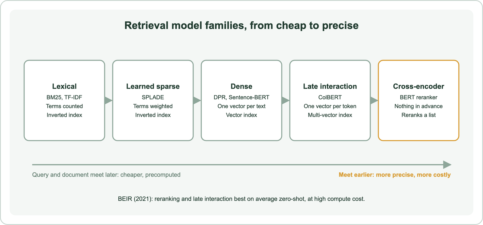
The main types of information retrieval models are classical lexical models, learned sparse models, dense models, late-interaction models, and cross-encoders. The classical group itself splits into Boolean, vector space, probabilistic, and language-model approaches, as Manning, Raghavan, and Schütze’s textbook “Introduction to Information Retrieval” lays out.
| Family | Representation | Example | Typical role |
|---|---|---|---|
| Boolean | Term presence | AND, OR, NOT queries | Exact filtering, no ranking |
| Vector space | Weighted term vectors | TF-IDF | Ranked keyword search |
| Probabilistic | Term statistics | BM25 | Default keyword ranking |
| Learned sparse | Learned term weights | SPLADE | First-stage retrieval with expansion |
| Dense | One vector per text | DPR, Sentence-BERT | First-stage semantic retrieval |
| Late interaction | One vector per token | ColBERT | Precise first stage or reranking |
| Cross-encoder | Joint query and document | BERT reranker | Reranking a shortlist |
The table runs roughly from cheapest to most expensive per comparison. The first three families are lexical: they need shared words. The last four are neural: they learn what counts as related. Retrieval as a stage is also different from generation, which some readers fold in under “types of retrieval.” The classical models still anchor almost every system, so they come first.
How do classical retrieval models rank documents?
Classical retrieval models rank documents by statistics about the words a query and document share. They need no training data. They run on an inverted index that maps each term to the documents containing it.
The Boolean model is the simplest. Manning and colleagues describe it as returning every document that satisfies a logical expression of terms. It does not rank. A document either matches or it does not, which suits strict filters and legal discovery but leaves the user to sort the results.
The vector space model adds ranking. Each document and query becomes a vector of term weights, usually TF-IDF. Term frequency rewards words that repeat in a document. Inverse document frequency rewards words that are rare in the collection. The score is the similarity of the two vectors.
Probabilistic models estimate how likely a document is to be relevant. BM25 is the best known. Robertson and Zaragoza’s 2009 review describes it as a term-weighting and scoring function from the probabilistic relevance framework. It limits how much a repeated term can add and normalizes for document length. Weaviate’s keyword search uses BM25F, a variant that scores across several fields. Language-model retrieval, another classical approach, ranks documents by how likely they are to generate the query. The keyword search guide covers these scoring details. All of them share one weakness: a relevant document that uses different words scores zero. Learned sparse models were built to fix that without leaving the inverted index.
How do sparse retrieval models work?
Sparse retrieval models represent each text as a long vector over the vocabulary in which almost every weight is zero, so they can be searched with an inverted index. BM25 is sparse in this sense. Learned sparse models keep the format but let a neural network choose the weights. Sparse retrieval covers the family in depth.
The key move is expansion. A learned sparse model can assign weight to words that do not appear in the text but are related to it. A document about “automobile repair” can gain weight on “car” and “mechanic.” That lets an exact-match index find documents that never used the query’s words.
SPLADE is the reference example. Formal, Piwowarski, and Clinchant’s SIGIR 2021 paper describes highly sparse representations produced with explicit sparsity regularization and log-saturated term weights. The authors note that the representations stay compatible with inverted indexes and keep exact term matching. They report results competitive with leading dense and sparse methods. SPLADE and learned sparse retrieval explains the training details.
Sparse models keep two advantages from the classical world. Their weights are inspectable, so a team can see which terms drove a match. They also reuse mature keyword infrastructure. Their limit is that meaning is still tied to vocabulary terms. Dense models drop that tie entirely.
How do dense retrieval models work?
Dense retrieval models encode each query and document into one fixed-length vector and retrieve the documents whose vectors are closest to the query’s. Every dimension carries some value, which is why the vectors are called dense. Dense retrieval is the mechanism behind most semantic search.
The standard architecture is the bi-encoder. A bi-encoder runs the query and the document through encoders separately, so document vectors can be computed once and stored. At query time, only the query is encoded. A vector index then finds the nearest stored vectors quickly.
Two papers set the pattern. Reimers and Gurevych’s 2019 Sentence-BERT trained networks so sentence embeddings could be compared by cosine similarity. Karpukhin and colleagues’ 2020 Dense Passage Retrieval trained a dual encoder for questions and passages and searched by maximum inner product. On its open-domain question-answering datasets, DPR beat a Lucene BM25 baseline by 9 to 19 points in top-20 passage retrieval accuracy.
Dense models handle paraphrase and vocabulary mismatch well. Their weakness is compression. A whole passage becomes one vector, so a rare name or code can be blurred. The BEIR benchmark by Thakur and colleagues found that dense models often underperform other approaches when moved to new domains without retraining. The dense versus sparse retrieval comparison weighs the two directly. Late interaction keeps more detail by refusing to compress so much.
How does late interaction retrieval work?
Late interaction retrieval keeps one vector for every token in the query and document, then scores a match by comparing each query token with its best-matching document token. Khattab and Zaharia introduced the approach with ColBERT at SIGIR 2020. ColBERT and late interaction covers the model family in detail.
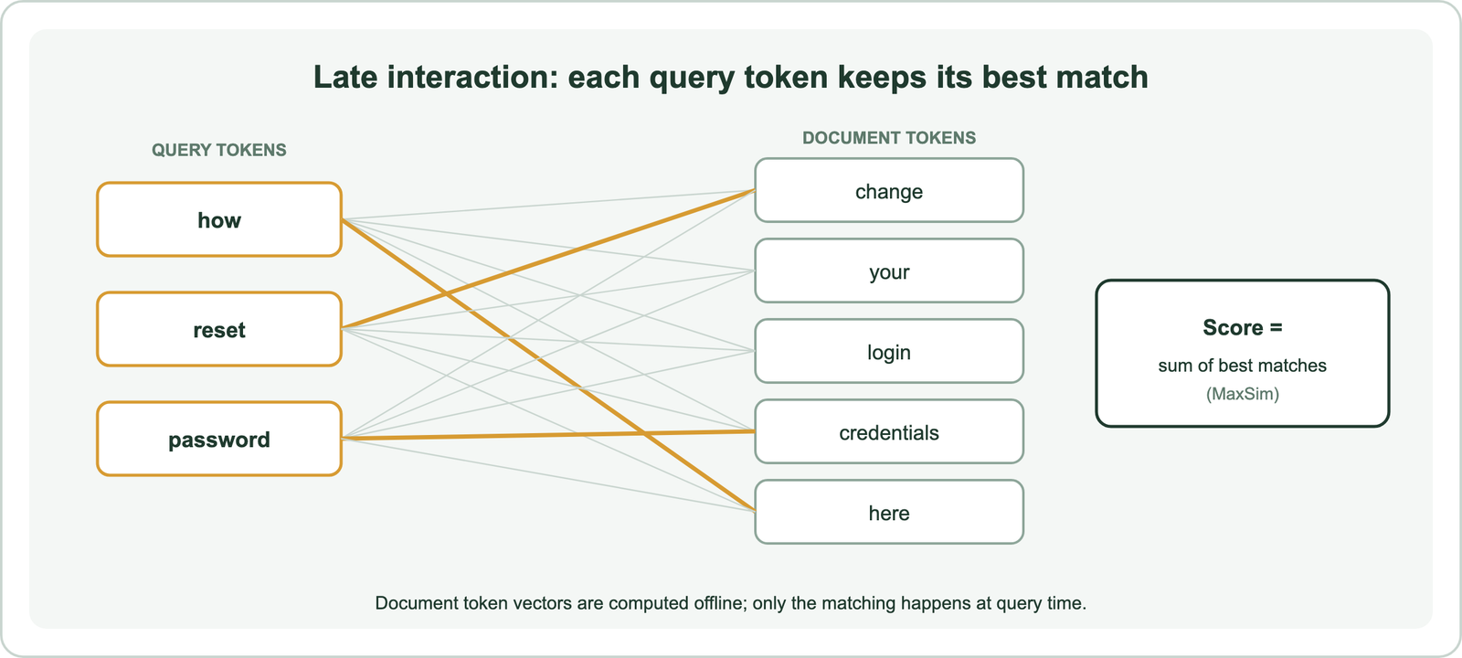
The scoring step is called MaxSim. For each query token, the model finds the most similar document token vector and keeps that similarity. The document’s score is the sum across query tokens. Because document token vectors are computed offline, the interaction happens “late,” only at query time. The ColBERT paper reports running two orders of magnitude faster than comparable BERT rankers, with four orders of magnitude fewer operations per query.
The cost is storage. A document with hundreds of tokens needs hundreds of vectors. Weaviate supports these multi-vector embeddings for ColBERT, ColPali, and ColQwen models, generally available since version 1.30. It notes that they can be much larger than single vectors. Weaviate’s MUVERA encoding, added in version 1.31, compresses each multi-vector into one fixed-length vector. In Weaviate’s test on the LoTTE dataset, MUVERA cut memory by about 70 percent and import time from over 20 minutes to 3 to 6 minutes, with some recall loss that higher ef settings can recover. Cross-encoders push interaction even earlier.
Where do cross-encoders fit among retrieval models?
Cross-encoders fit at the precise end of the spectrum: they read the query and document as one input and output a relevance score, so they rerank a shortlist rather than search a collection. Because the score depends on both texts at once, nothing can be computed in advance. Weaviate’s reranking documentation notes this is why cross-encoders run as a second stage.
A cross-encoder sees every interaction between query and document words. That makes it the most accurate single comparison in this list. It also makes it the most expensive, because one model pass runs for every candidate on every query.
The bi-encoder versus cross-encoder comparison sets out the split. Bi-encoders retrieve, cross-encoders rerank. A typical pipeline retrieves candidates with BM25, a dense model, or both, and then lets a cross-encoder reorder them. Reranking covers that stage, including its latency cost and the limit that it cannot recover a missed candidate.
The same idea extends to agents. Agentic retrieval uses a language model to plan several searches, read results, and decide what to fetch next. It is a control loop around retrieval models rather than a new representation. With every family placed, a direct comparison becomes possible.
How do the retrieval model families compare?
Retrieval model families compare on what they precompute, how they index, what they match well, and what each query costs. No family wins on every axis. The best evidence for that comes from a benchmark designed to test models outside their training data.
| Family | Precomputed | Index | Matches well | Main cost |
|---|---|---|---|---|
| BM25 | Term statistics | Inverted index | Exact terms, names, codes | Misses paraphrases |
| Learned sparse | Learned term weights | Inverted index | Exact terms plus expansions | Model inference at indexing |
| Dense | One vector per text | Vector index | Paraphrase, meaning | Can blur rare terms |
| Late interaction | One vector per token | Multi-vector index | Fine-grained matches | Much more storage |
| Cross-encoder | Nothing | None (reranks a list) | Full query-document interplay | One model pass per candidate |
The table shows a trade between precomputation and precision. Thakur and colleagues’ BEIR benchmark, presented at NeurIPS 2021, tested models zero-shot across 18 datasets. It found BM25 a robust baseline. Reranking and late-interaction models achieved the best zero-shot performance on average, but at high computational cost. Dense and sparse models were more efficient but often underperformed.
That result does not crown a winner. It says that cheap models generalize unevenly, and expensive models generalize better but cost more.
Operations differ as much as accuracy. A BM25 index updates cheaply, because adding a document only adds its terms to the postings lists. Learned sparse and dense indexes need a model pass for every new or changed document before it can be found. Late-interaction indexes need a pass and many more vectors. Changing the model is the heaviest operation of all: dense, sparse, and late-interaction vectors from an old model cannot be compared with vectors from a new one, so every stored item must be encoded again. Interpretability also varies. A BM25 or SPLADE score can be traced to specific terms, while a dense score comes from a learned space that resists inspection. These operating differences often decide the choice once accuracy is close. Most production systems resolve the whole trade by combining families.
How should a team choose a retrieval model?
A team should choose a retrieval model by its queries, and usually combines keyword and dense models in hybrid search, with a reranker when precision justifies the cost. Weaviate’s hybrid search runs BM25 and vector search in parallel and fuses the results. Its alpha parameter runs from 0, keyword only, to 1, vector only. The hybrid search guide explains the fusion.
A practical sequence keeps the choice evidence-based:
- Start with BM25 as a baseline, since BEIR found it robust.
- Add a dense model and test hybrid fusion on judged queries.
- Try learned sparse or late interaction where exact terms and nuance both matter.
- Rerank the top candidates with a cross-encoder if precision at the top is critical.
- Measure recall, ranking quality, latency, and memory at every step.
Some design choices sit beside the model. Small-to-big retrieval matches on small chunks and then returns their larger parent section, a chunking pattern covered in chunking for semantic search. Combining structured filters with vector search is covered in metadata filtering.
Retrieval models also power retrieval-augmented generation. RAG means a system retrieves relevant passages and gives them to a large language model, or LLM, as context for its answer. The retrieval model decides which evidence the LLM sees, so its quality caps the answer’s quality. Semantic search in RAG explains that pipeline for beginners and practitioners alike.
A retrieval model is the method a search system uses to represent queries and documents and to score their match. Classical models such as BM25 score shared words and remain robust baselines. Learned sparse models add expansion, dense models capture meaning in one vector, late-interaction models keep a vector per token, and cross-encoders read query and document together. Each step toward earlier interaction buys precision with cost. The decision is to start from BM25, add dense retrieval through hybrid search, rerank where the top results matter most, and keep only what measurably improves judged results within the latency and memory budget.