Home / Foundations / Latent Semantic Indexing (LSI) Explained

Latent Semantic Indexing (LSI) Explained

Latent semantic indexing (LSI) is a retrieval method from the late 1980s that finds hidden topics in a collection by factorising its term-document matrix with singular value decomposition and keeping only the strongest dimensions. Documents and queries are then compared in that small topic space instead of by shared words, so a query for “automobile” can match a document that only says “car”. LSI was introduced by Deerwester, Dumais, Furnas, Landauer and Harshman, published in 1990, and was one of the first practical answers to the vocabulary mismatch problem. It represents each document as a dense vector compared by cosine similarity, an idea that modern embeddings inherited. Its weaknesses, including expensive updates, linear structure and no sense of word order, led to its replacement by probabilistic topic models and then neural embeddings. “LSI keywords”, a term used in some SEO advice, has nothing to do with how modern search engines work.

What is latent semantic indexing?

Latent semantic indexing is a technique that represents documents and terms as vectors in a reduced space of latent topics, derived from word co-occurrence, so retrieval can match meaning rather than exact words. It is also called latent semantic analysis when used outside retrieval.

The starting point is a term-document matrix. Each row is a term, each column a document, and each cell counts how often the term appears in the document, usually with a weighting such as TF-IDF. This is the representation of the vector space model, in which documents are compared by the terms they share.

LSI compresses that matrix. Using singular value decomposition, it finds the directions along which documents vary most, keeps a few hundred of them and discards the rest. Each document becomes a short dense vector over those latent dimensions. Terms that tend to appear in the same documents, such as “car” and “automobile”, end up pointing the same way.

The word “latent” refers to those hidden dimensions. Nobody labels them; they emerge from the statistics of the collection. Retrieval then compares a query vector with document vectors in the latent space, typically by cosine similarity.

Who is credited with inventing latent semantic indexing?

Latent semantic indexing was developed by Scott Deerwester, Susan Dumais, George Furnas, Thomas Landauer and Richard Harshman, and described in their 1990 paper “Indexing by Latent Semantic Analysis”. Much of the work was done at Bellcore.

The team was addressing a problem they had studied in human behaviour: people use many different words for the same thing, so keyword retrieval often misses relevant documents. Furnas and colleagues had earlier shown how rarely two people choose the same word for a concept. LSI was an attempt to recover the shared concept behind the varied words, statistically and without a hand-built thesaurus.

A patent on the method was filed in 1988, and the 1990 paper in the Journal of the American Society for Information Science became one of the most cited works in information retrieval. The broader field is introduced in what is information retrieval.

How does latent semantic indexing work?

Latent semantic indexing works by decomposing the term-document matrix A into U, S and V-transpose with SVD, keeping the k largest singular values, and using the truncated factors as term and document coordinates. The truncation is what creates the topic space.

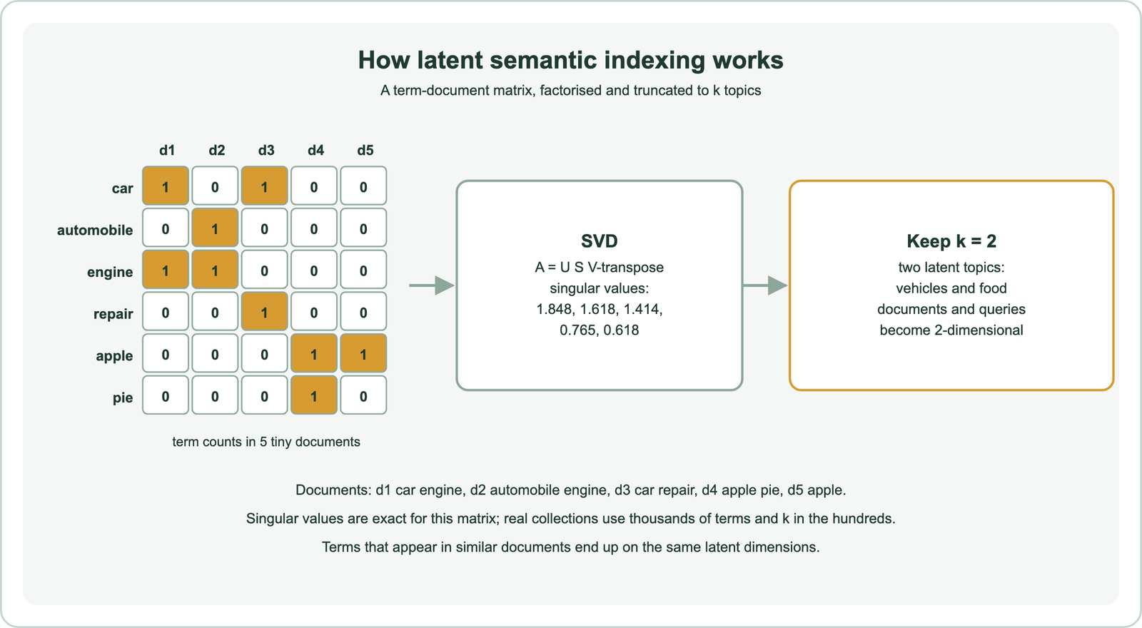
Singular value decomposition writes any matrix as a product of three: U holds term coordinates, S is a diagonal matrix of singular values in decreasing order, and V holds document coordinates. Each singular value measures how much of the matrix’s structure its dimension explains. Keeping only the largest k gives the best rank-k approximation of the original matrix in the least-squares sense.

In the toy example, five short documents about vehicles and food give singular values of 1.848, 1.618, 1.414, 0.765 and 0.618. Keeping the first two separates the collection into a vehicle topic and a food topic. In real collections, k is typically set to a few hundred, and choosing it is an empirical decision: too small merges distinct topics, too large keeps noise.

How does LSI match a query to documents?

LSI matches a query to documents by projecting the query’s term vector into the latent space, then ranking documents by cosine similarity with it. Shared topics count even without shared words.

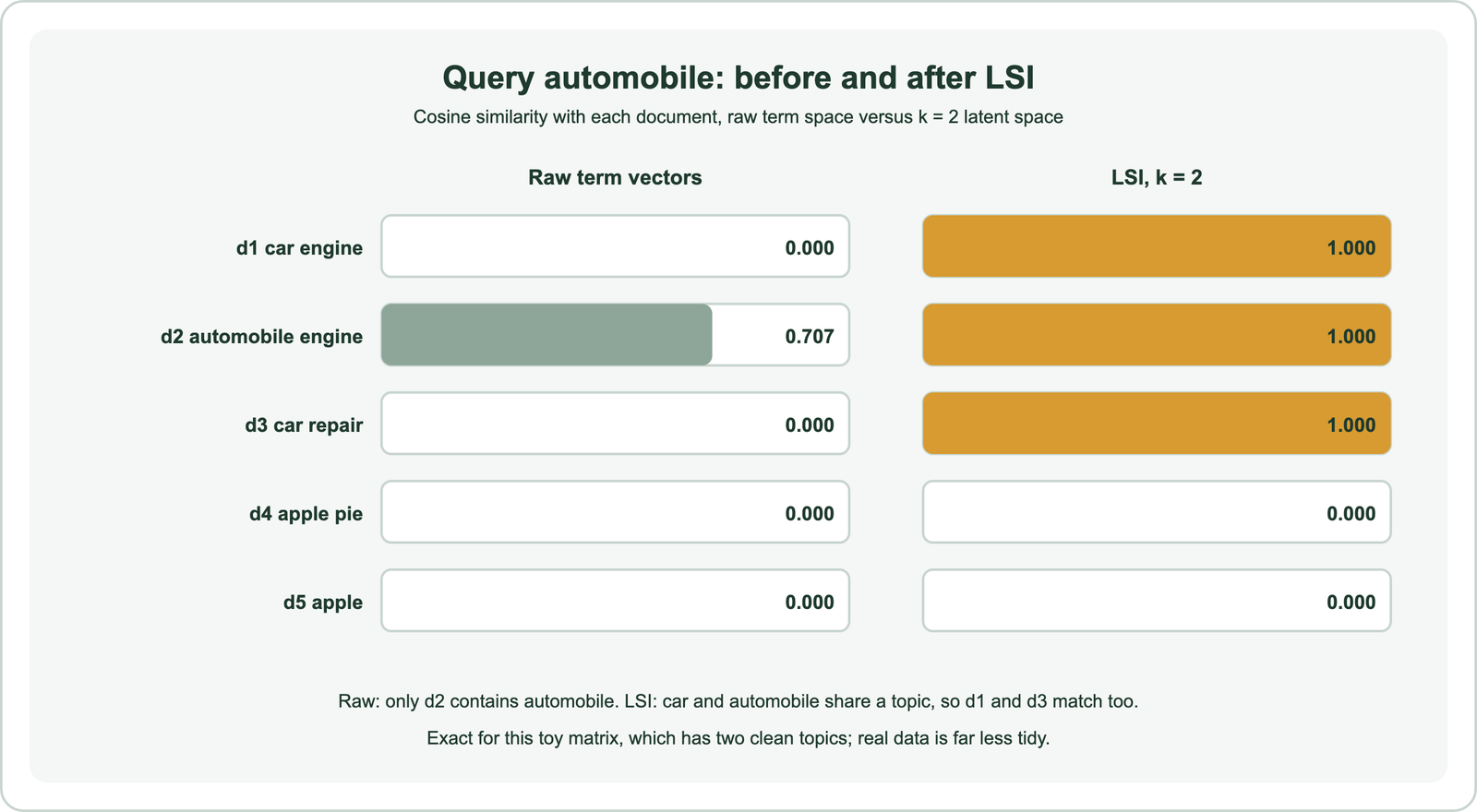
The projection, often called folding in, multiplies the query’s term vector by the first k columns of U and divides by the matching singular values. The result lives in the same k-dimensional space as the documents. Documents never seen at decomposition time can be folded in the same way.

The toy example shows the effect. In raw term space, the query “automobile” has a cosine of 0.707 with “automobile engine” and 0 with every other document, including “car engine”. In the two-dimensional latent space, it scores 1.000 with all three vehicle documents and 0 with the food documents. “Car” and “automobile” never appear together, but both co-occur with “engine”, which ties them to the same topic. The perfect scores are an artefact of the tiny, clean example.

Which search problems does LSI solve?

LSI addresses synonymy, where different words name the same concept, and reduces noise from incidental word choices, which improves recall over plain keyword matching. It handles polysemy only partly.

Synonymy was the main target. Keyword search fails when a query and a relevant document use different words, a failure described in the vocabulary mismatch problem. By mapping co-occurring terms to shared dimensions, LSI let queries match documents that used related vocabulary.

Polysemy, one word with several meanings, was harder. A word like “bank” gets a single vector in LSI, placed somewhere between its senses, so the method can only partly separate them through the other words in a query. Distinguishing what words mean from what they merely co-occur with is the subject of semantic similarity vs relatedness.

Why have newer methods replaced LSI?

Newer methods replaced LSI because its decomposition is expensive to compute and update, its linear model cannot capture word order or context, and probabilistic and neural methods produced better representations. It remains a useful teaching example.

Updating is the practical problem. New documents can be folded in, but they do not change the latent space, so as a collection grows the space drifts out of date and must be recomputed. Full SVD on a large, sparse matrix is costly, which limited LSI to collections that changed slowly.

Models improved on its statistics. Probabilistic latent semantic analysis, by Hofmann in 1999, recast topics as probability distributions. Latent Dirichlet allocation, by Blei, Ng and Jordan in 2003, added a full generative model of documents. Neural word embeddings followed, covered in word2vec and GloVe, and then contextual models, covered in transformers and BERT in search and Sentence-BERT. Weaviate’s article on embedding model change traces the same progression from static word vectors to context-aware ones.

Are LSI keywords real?

LSI keywords are not real in the sense that SEO advice suggests: there is no public evidence that modern search engines use latent semantic indexing, and a Google representative has said so directly. The term is a misnomer for related words.

The phrase spread through SEO content as a label for synonyms and related terms that supposedly signal relevance to search engines. Google’s John Mueller wrote publicly in 2019 that there is no such thing as LSI keywords. LSI itself is a 1980s method designed for small, static collections, and its update costs make it a poor fit for an index of the web.

Covering a topic with its natural vocabulary still helps readers and search engines understand a page, but that is a matter of writing well about a subject, not of a specific algorithm. How Google has publicly described its own semantic systems is covered in semantic search at Google.

How do you compute LSI in Python?

You compute LSI in Python by building a term-document matrix, running a singular value decomposition, keeping k components, and folding queries into the same space. NumPy is enough for small examples.

import numpy as np

terms = ["car", "automobile", "engine", "repair", "apple", "pie"]
docs = ["car engine", "automobile engine", "car repair", "apple pie", "apple"]
A = np.array([[d.split().count(t) for d in docs] for t in terms], float)

U, s, Vt = np.linalg.svd(A, full_matrices=False)
k = 2
Uk, sk, Vk = U[:, :k], s[:k], Vt[:k].T            # term coords, singular values, doc coords

q = np.array([t == "automobile" for t in terms], float)
q_hat = q @ Uk / sk                                 # fold the query into the latent space
cos = lambda a, b: a @ b / (np.linalg.norm(a) * np.linalg.norm(b))
print([round(cos(q_hat, Vk[j]), 3) for j in range(len(docs))])   # [1.0, 1.0, 1.0, 0.0, 0.0]

The script was run to compute the worked example and reproduces the values in both figures. For real collections, libraries such as scikit-learn offer truncated SVD on sparse matrices, and TF-IDF weighting usually replaces raw counts.

The same idea of dense vectors compared by cosine now runs at scale in vector databases. The reasons dense spaces work despite many dimensions are discussed in the curse of dimensionality and high-dimensional vector space.

How does LSI relate to modern semantic search?

LSI anticipated modern semantic search by representing documents as dense vectors that capture meaning and comparing them by cosine similarity. Modern embeddings learn those vectors from far more data with neural networks.

The lineage is direct. LSI showed that a compressed space learned from co-occurrence could match related words, and every later method refined that idea. Word2vec learned word vectors from local context windows, transformers added context and order, and sentence embedding models trained vectors specifically for retrieval. Today’s vector databases, such as Weaviate, store and search those vectors at scales LSI could not reach.

Structured knowledge took a parallel path, described in knowledge graphs in search. Caching and other systems concerns are covered in cache hits and misses.

Latent semantic indexing factorises a term-document matrix with SVD, keeps the strongest k dimensions, and compares documents and queries in that topic space, so related words can match even when they never appear together. Introduced by Deerwester and colleagues in 1990, it addressed synonymy and introduced dense document vectors compared by cosine, an idea modern embeddings inherited. Its costly updates, linear structure and blindness to word order led to topic models and then neural embeddings. “LSI keywords” is an SEO misnomer that Google has publicly rejected; good topical coverage helps, but not because of LSI.