Home / How it works / Exact vs Approximate Nearest Neighbor Search: The Trade-off

Exact vs Approximate Nearest Neighbor Search: The Trade-off

Exact nearest neighbor search compares a query with every stored vector and always returns the true closest matches. Approximate nearest neighbor (ANN) search checks only a promising subset, trading a little recall for much faster queries. Exact search, often called a flat index or brute force, is the right choice for small collections, heavily filtered subsets, and for measuring the accuracy of an ANN index. Its cost grows in direct proportion to the collection: one query over a million 768-dimension vectors needs 768 million multiply-adds. ANN indexes such as HNSW graphs and IVF lists visit a small fraction of vectors instead, with settings that trade speed against recall. Weaviate offers both, plus a dynamic index that starts flat and switches to HNSW at a threshold, 10,000 objects by default.

What is the difference between exact and approximate nearest neighbor search?

The difference is that exact search guarantees the true top-k results by checking every vector, while approximate search checks far fewer vectors through an index. Its results are usually, but not always, the true top-k. The trade is recall for speed.

Nearest neighbor search is the core operation of vector search: given a query vector, find the stored vectors closest to it. “Closest” is defined by a distance measure, as described in cosine vs dot product vs Euclidean distance. Exact search computes that distance for every stored vector, sorts, and returns the top k. Nothing can be missed.

Approximate search builds a data structure ahead of time that lets the query skip most of the collection. It might walk a graph towards the query, or search only the clusters nearest to it. Occasionally a true neighbour sits somewhere the search did not look, and it is missed. The share of true neighbours found is called recall, and ANN recall covers how to measure it.

How much work does exact search do per query?

Exact search does one distance calculation per stored vector per query, so its work equals the number of vectors times the number of dimensions. Doubling the collection doubles the cost.

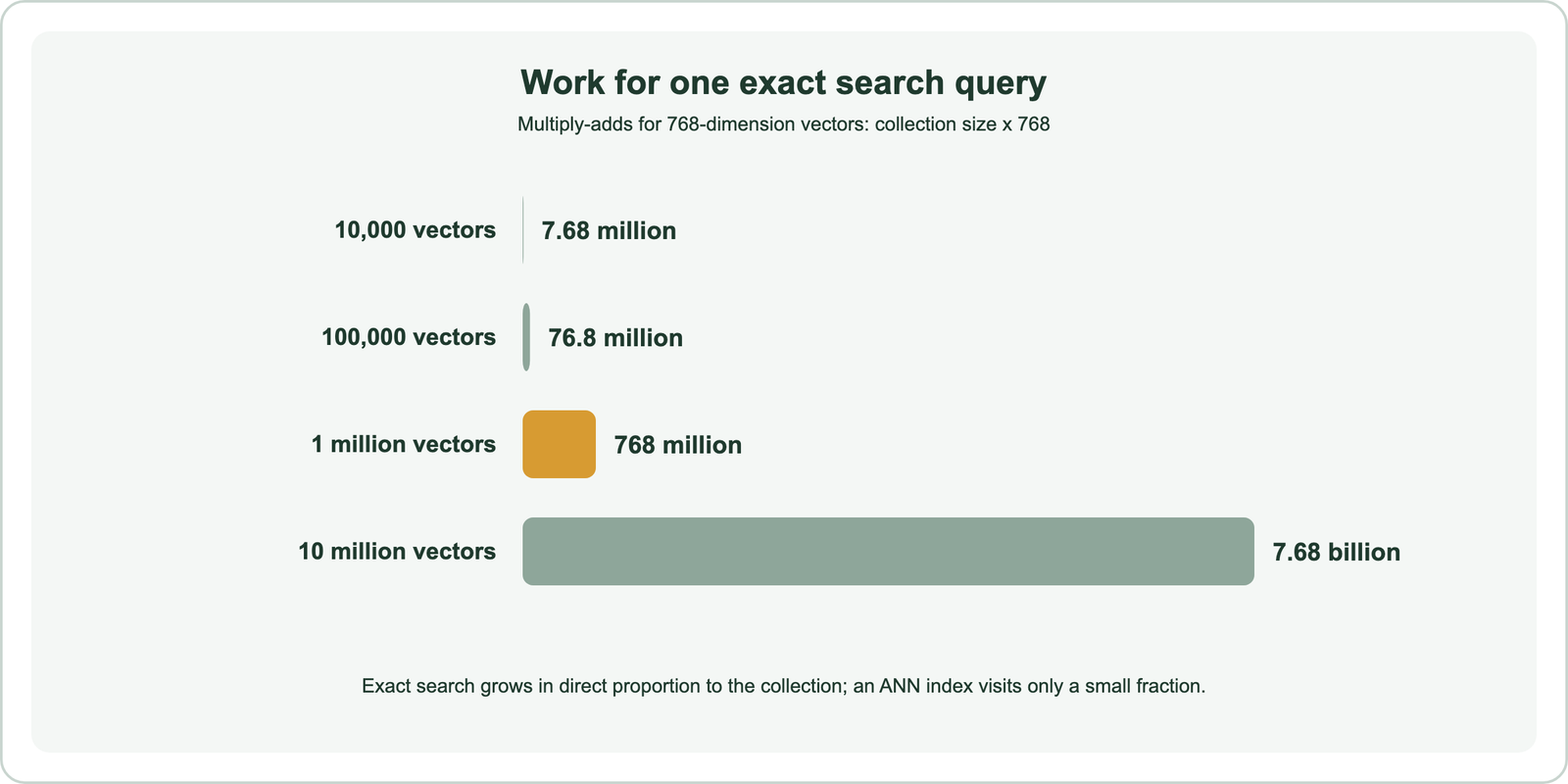
A dot product of two 768-dimension vectors takes 768 multiply-adds. Over 10,000 vectors that is 7.68 million per query, which a modern processor handles quickly. Over 10 million vectors it is 7.68 billion per query, and that cost repeats for every query and every concurrent user. Memory bandwidth also becomes a limit, since every vector must be read for every query.

Exact search gets faster with hardware and compression but never changes shape. Vectorised CPU instructions, GPUs and quantized vectors all cut the constant, which is why brute force with binary or 8-bit vectors can stay practical for larger sets than raw floats. The work still grows in a straight line with the data, whereas ANN indexes grow far more slowly.

When is exact search the right choice?

Exact search is the right choice for small collections, for queries restricted by filters to a small subset, for evaluation baselines, and where missing any true match is unacceptable. It is simple, precise and cheap on memory.

Small collections need no index. Weaviate’s documentation describes the flat index as ideal for small object counts, with lower memory overhead and good latency. Its tutorial suggests flat for indexes of about 10,000 to 20,000 objects, while its academy course places the switch near 100,000. The right point depends on dimensions, hardware and latency targets, so measure it. Multi-tenant systems with many small tenants are the classic flat-index case.

Exact search also wins when a filter shrinks the candidates. If a query is limited to one user’s 2,000 documents, scanning those 2,000 exactly beats walking a graph built for millions. Finally, exact search is the reference for every ANN benchmark: you cannot measure recall without knowing the true neighbours. Similarity search covers the general problem.

How does approximate nearest neighbor search reduce the work?

Approximate nearest neighbor search reduces the work by organising vectors into a structure, such as a graph or a set of clusters, that leads each query to a small, promising part of the collection. Different index families organise the space differently.

HNSW, the default in Weaviate, builds a layered graph in which each vector links to near neighbours. A query starts at the top layer and moves greedily towards closer vectors, dropping to denser layers as it goes. IVF indexes cluster vectors into lists around centroids, then search only the lists whose centroids are closest to the query. Both visit a small fraction of the collection.

Each family exposes a knob that trades speed for recall. In HNSW it is ef, the size of the candidate list during search; Weaviate’s documentation notes diminishing recall gains above 512. In IVF it is the number of lists probed. Approximate nearest neighbor search covers the algorithms, and semantic indexing and vector indexes covers how they fit into a search system.

What is an IVFFlat index?

An IVFFlat index is an approximate index that divides vectors into lists around cluster centroids and searches only the lists closest to the query, comparing full vectors within them. “Flat” means the vectors inside each list are stored uncompressed.

pgvector, the Postgres extension, offers IVFFlat and HNSW. Its documentation says pgvector performs exact search by default, with perfect recall, and uses approximate search only once an index is added. For IVFFlat it advises creating the index after the table has data. A starting point for lists is rows divided by 1,000 up to a million rows, and the square root of rows above that. For probes, start at the square root of lists.

Probes default to 1 and can be raised per query; setting probes equal to lists amounts to exact search. pgvector’s documentation also states that HNSW gives a better speed-recall trade-off than IVFFlat, while IVFFlat builds faster and uses less memory. Setup details are in semantic search with Postgres and pgvector.

What are the pros and cons of HNSW versus a flat index?

HNSW’s pros are fast queries at almost any scale and tunable recall; its cons are higher memory use, slower imports and results that are approximate. A flat index is the reverse. Collection size usually decides.

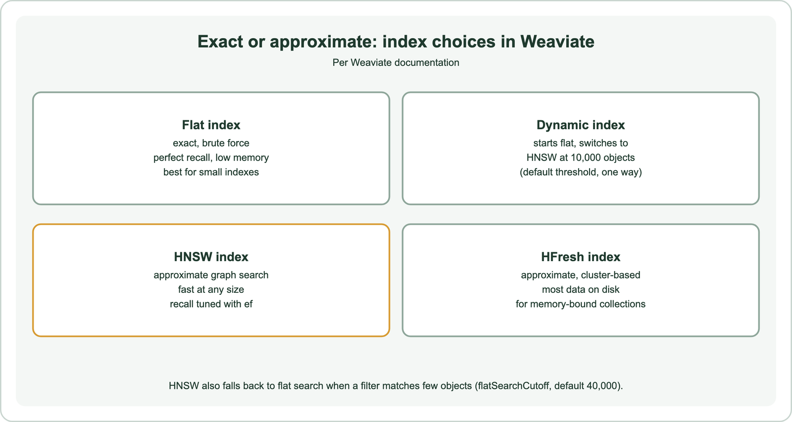
An HNSW index keeps its graph and vectors in memory for speed, and it must insert each new vector into the graph, which slows imports. A flat index stores vectors with almost no extra structure and scans them at query time. Weaviate’s dynamic index starts flat and builds HNSW once a collection or tenant passes a threshold, 10,000 objects by default. The conversion is one way and requires asynchronous indexing.

Weaviate also mixes the two inside HNSW. When a filter matches fewer objects than the flatSearchCutoff setting, 40,000 by default, the search switches to an exact scan of the matching objects. Very restrictive filters make graph traversal nearly exhaustive, so scanning the small subset is faster. Top-k retrieval explains how the final list is cut.

How do you measure what approximation costs?

You measure what approximation costs by running the same queries through exact search and the ANN index, and computing recall at k: the share of the true top-k that the index returned. Pair it with latency at the same settings.

Take a sample of real queries. For each, compute the exact top 10 with a flat scan, then the ANN top 10, and count the overlap. Repeat across settings such as ef or probes, and plot recall against latency. Choose the cheapest setting whose recall your application accepts. Recheck after large data changes, compression or a new embedding model.

Recall measures fidelity to exact search, not relevance to users. A perfect ANN index can still return poor results if the embeddings are weak, which is a different problem covered in relevance scores. Keep the two measurements separate so a model problem is not blamed on the index, or the reverse.

How does the choice fit into a semantic search system?

The choice of exact or approximate search is one layer of a semantic search system, sitting between the embeddings that represent meaning and the ranking that orders results. It affects speed and recall, not what the vectors mean.

The same choice appears for dense vectors, which need ANN indexes at scale, and sparse vectors, which use inverted indexes instead, as compared in dense vs sparse vectors. Upstream choices such as chunking set how many vectors there are, and so how soon an index is needed.

Search quality comes from the layers working together. Semantic matching, synonyms and related terms and multilingual search depend on the embeddings. The index only decides how fast and how faithfully those embeddings are searched. How semantic search works and semantic search architecture show the full picture.

Exact nearest neighbor search checks every vector and always finds the true matches; approximate search checks a small, well-chosen subset and usually does. Exact work grows linearly, 768 million multiply-adds per query for a million 768-dimension vectors, so large collections need ANN indexes such as HNSW or IVF. Use flat indexes for small collections, small tenants and heavily filtered subsets, and keep exact search as the yardstick for measuring ANN recall. In Weaviate, choose flat, HNSW, dynamic or HFresh by collection size and memory, and tune recall against latency on real queries.