Home / Scale and cost / Recall vs Latency: The Core Trade-off in Semantic Search
Decision guideRecall vs Latency: The Core Trade-off in Semantic Search
The recall versus latency trade-off is the core tuning choice in semantic search: approximate vector indexes answer faster by checking fewer vectors, and checking fewer vectors means sometimes missing a true nearest neighbor. Recall is the share of the true top results an index returns; latency is how long it takes. Index settings move a system along a curve between the two. For HNSW the main dials are ef at query time and maxConnections and efConstruction at build time. Weaviate’s starting values are ef 64, efConstruction 128, and maxConnections 32. In this site’s test, raising the search list from 256 to 512 cost about 80 percent more work and added no recall. Plot the curve on your own data and stop where extra recall stops paying.
Recall versus latency in four facts
- Exact search is perfectly accurate but scales linearly; approximate indexes trade a little recall for large speed gains.
- Query-time
efmoves you along the curve; build-time graph degree sets how high the curve can reach. - Weaviate’s SIFT1M benchmark reaches 98.35 percent recall@10 at 1.44 ms mean and 3.13 ms p99 latency.
- Compression shifts the curve: rescoring the top 20 int8-compressed candidates restored 0.995 recall in our test.
What is the recall versus latency trade-off?
The recall versus latency trade-off is the relationship, in approximate nearest neighbor search, between how many of the true nearest neighbors a query returns and how long the query takes. Higher recall almost always costs more time.
Recall@k compares an index’s top k results with the exact top k. If exact search would return ten documents and the index returns eight of them, recall@10 is 0.8. Weaviate’s FAQ puts it plainly: a 98 percent recall means 2 percent of results will not match the true nearest neighbors. ANN recall covers how to measure it.
Latency is the time a query takes, usually reported as a mean and a tail percentile such as p99. Throughput, in queries per second, is the related capacity measure. Vector database benchmarks plot recall against throughput or latency as a curve, and every index setting is a point on it. Search latency covers the other contributors to response time.
Why does approximate search trade recall for speed?
Approximate search trades recall for speed because comparing a query with every stored vector grows linearly with the data, while an index that inspects only a small, promising fraction can occasionally skip a true neighbor. The trade is deliberate.
Exact search is simple and always correct. In this site’s timing test, exact search over 100,000 normalized 384-dimensional vectors took 2.3 ms on a laptop CPU, and over 1 million took 21.3 ms. Growth stays linear: ten times the data, ten times the time. Weaviate’s binary quantization article makes the same point, noting brute force at 1 million vectors runs roughly ten times slower than at 100,000.
A graph index like HNSW avoids that growth by walking from node to node toward the query, comparing only the vectors along the way. Weaviate’s documentation describes sub-50 ms queries for 20 nearest neighbors on datasets of 1 to 100 million objects. The cost is that a walk can stop at a good-but-not-best region. Approximate nearest neighbor search explains the families of indexes.
What does a recall-latency curve look like?
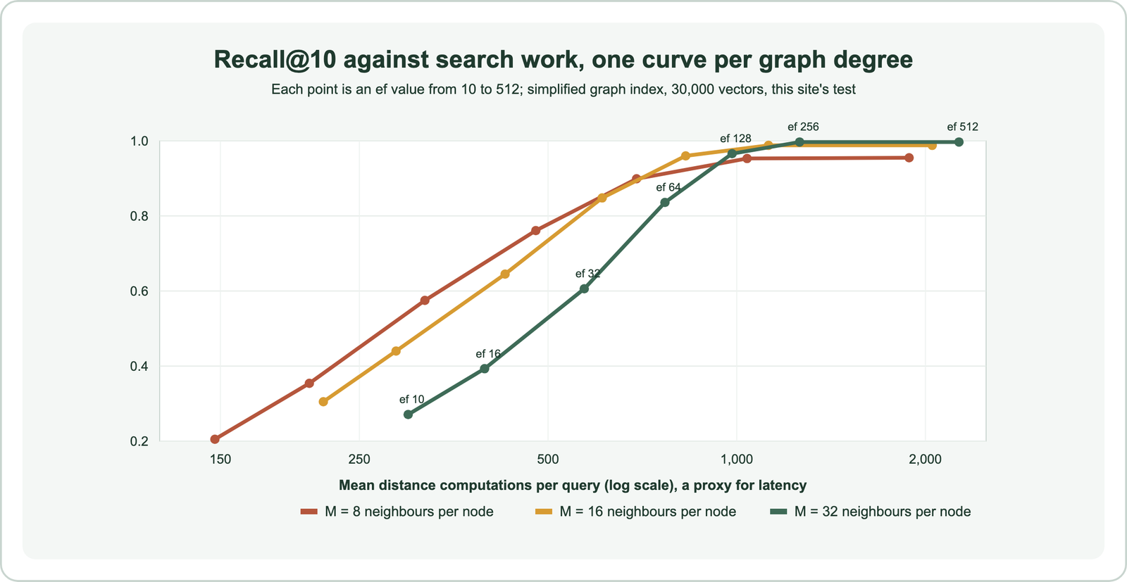
A recall-latency curve rises steeply at first, as small increases in search effort bring large recall gains, then flattens as each extra point of recall costs more and more work. We plotted one with a simplified graph index.
The test used 30,000 vectors in 96 dimensions, grouped into 100 clusters, with 200 queries and k of 10. The index was a single-layer navigable graph, each node linked to its M nearest neighbors plus two random long links. That is a simplified stand-in for HNSW’s bottom layer, not Weaviate’s implementation. We varied the search list size, ef, from 10 to 512 and counted distance computations, the work that dominates latency.
| ef | Recall@10 | Mean distance computations | p99 distance computations |
|---|---|---|---|
| 10 | 0.305 | 219 | 412 |
| 32 | 0.645 | 427 | 802 |
| 64 | 0.848 | 610 | 1,091 |
| 128 | 0.960 | 829 | 1,571 |
| 256 | 0.988 | 1,124 | 1,931 |
| 512 | 0.988 | 2,051 | 2,600 |
The shape is the important part. Going from ef 32 to 64 raised recall by 0.20 for 43 percent more work. Going from 256 to 512 raised it by nothing for 82 percent more work. Exact search over all 30,000 vectors would cost 30,000 distance computations per query, so even the most expensive setting did a fifteenth of that work.
How does ef change recall and latency?
The ef setting changes recall and latency by setting how many candidates the search keeps in its list while it walks the graph. A larger list explores more paths, finds more true neighbors, and takes longer. It is the main query-time dial for HNSW.
Weaviate’s documentation describes ef as the size of the dynamic list used during search, and notes that values above 512 show diminishing improvements in recall. Our curve flattened earlier, at 256, on a smaller dataset. Because ef is mutable, you can change it on a live collection without rebuilding the index.
Weaviate also offers dynamic ef, its default, set by ef of -1. The list size becomes the query limit times dynamicEfFactor, bounded by dynamicEfMin and dynamicEfMax, which default to 8, 100, and 500. A limit of 20 therefore gives an ef of 160. Weaviate’s FAQ notes a side effect: changing the limit changes ef, so result quality can shift with page size.
The fix, per the same FAQ, is to set a fixed ef that gives the recall you need. If recall varies a lot with ef, the documentation suggests stronger build parameters instead.
How do maxConnections and efConstruction change the curve?
The build parameters maxConnections and efConstruction change the curve itself, raising the recall it can reach, while ef only moves along it. They cost memory and import time instead of query time.
The sweep shows the ceiling effect. With 8 neighbors per node, recall stalled at 0.955 even at ef 512. With 16 it reached 0.988, and with 32 it reached 0.997. Denser graphs cost more per query at the same ef, because each node has more neighbors to check, but they reach recall a sparse graph never will.
Weaviate lowered its default maxConnections from 64 to 32 in version 1.26, after testing showed better QPS-recall curves for modern high-dimensional datasets. Its release notes put the best values in the 16 to 32 range, depending on dataset size. efConstruction, 128 by default, sets how thoroughly the graph is built; higher values improve the graph but slow imports. Unlike ef, both are fixed once the collection exists.
Weaviate’s configuration tips map these choices to workload. High query volume calls for a low ef, with recall raised through efConstruction if imports are rare. Heavy imports call for a low efConstruction, with recall raised through ef if queries are few. When both are high, raise efConstruction as far as import time allows, then tune ef.
What do Weaviate’s benchmarks show?
Weaviate’s benchmarks show that well-tuned HNSW reaches 96 to 98 percent recall@10 at single-digit millisecond latency on datasets from 1 million to 10 million vectors. The recommended configurations balance recall, latency, and throughput.
| Dataset | Size and dimensions | efC / maxConn / ef | Recall@10 | QPS | Mean latency | p99 latency |
|---|---|---|---|---|---|---|
| SIFT1M | 1M, 128 | 256 / 32 / 64 | 98.35% | 10,940 | 1.44 ms | 3.13 ms |
| DBPedia OpenAI | 1M, 1536 | 256 / 16 / 96 | 97.24% | 5,639 | 2.80 ms | 4.43 ms |
| MSMARCO Snowflake | 8.8M, 768 | 384 / 32 / 48 | 97.36% | 7,363 | 2.15 ms | 3.69 ms |
| Sphere DPR | 10M, 768 | 384 / 32 / 96 | 96.06% | 3,523 | 4.49 ms | 7.73 ms |
The benchmark measures end-to-end requests, including network time within one cloud network and retrieving full objects from disk. Weaviate notes this differs from ann-benchmarks, where embedded libraries return only IDs. Throughput figures come from a 30-core machine running many queries in parallel.
The benchmark’s own advice is to pick the dataset closest to your workload, read the expected recall and latency, and fine-tune from there. The benchmarking code is open source, so the numbers can be reproduced on your own hardware.
How does quantization change the trade-off?
Quantization changes the trade-off by compressing vectors so more fit in memory and distance computations run faster, at a small recall cost that rescoring with the original vectors can recover. It adds a third axis: memory.
Weaviate’s documentation lists typical savings and recall. Scalar quantization uses 75 percent less memory with 95 to 97 percent recall. 8-bit rotational quantization also saves 75 percent with 98 to 99 percent recall. Binary quantization saves 97 percent, with recall that varies by data. To offset the loss, Weaviate over-fetches candidates using compressed vectors, then rescores them with the uncompressed ones.
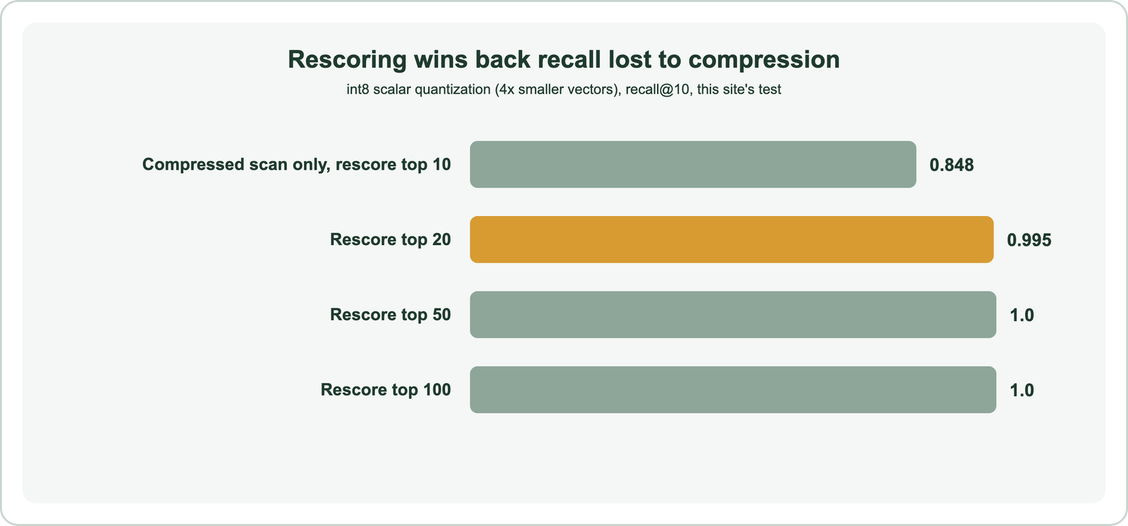
Our test compressed the same 30,000 vectors to 8-bit integers, four times smaller, and scanned them exactly. Taking the compressed top 10 directly gave 0.848 recall. Rescoring the compressed top 20 with the original vectors gave 0.995, and top 50 gave 1.000. A modest over-fetch recovered almost everything.
Compression can even improve the curve. Weaviate’s 8-bit rotational quantization article reports 15 to 50 percent higher throughput than uncompressed vectors, with recall dropping by less than a point at the same ef. With rescoring, it reached 99.41 percent recall at 2,738 QPS against 1,927 QPS uncompressed. Scaling semantic search covers memory planning.
Why does p99 latency matter more than the average?
The p99 latency matters more than the average because users notice the slowest queries, and approximate search has a long tail: some queries need far more work than typical ones to reach the same recall. Averages hide that spread.
In our test at M 16 and ef 128, the mean query needed 829 distance computations, but the 99th percentile needed 1,571, almost twice as many. Recall had a tail too. Even when average recall reached 0.96, the worst single query still scored 0.0 until ef rose to 256. Some queries start far from their answers and need a bigger search list to get there.
Weaviate’s benchmark reports p99 beside the mean for the same reason. On Sphere DPR, the mean latency was 4.49 ms and p99 was 7.73 ms. Set latency targets on p99, and check recall on the worst queries as well as the average. Search latency covers tail behavior in more depth.
How do you plot the curve for your own data?
You plot the curve for your own data by computing exact results for a sample of real queries, then running the same queries at several ef values and recording recall and latency for each. It takes an afternoon and replaces guesswork.
- Sample queries: take 200 to 1,000 real query vectors from logs.
- Compute ground truth: run exact search for each, with a flat index or brute force over a copy of the data.
- Sweep ef: run the queries at ef values such as 16, 32, 64, 128, 256, and 512.
- Record: recall@k against ground truth, mean and p99 latency, and the worst query’s recall.
- Pick the knee: choose the smallest ef that meets your recall target at your p99 budget.
import time
import weaviate
from weaviate.classes.config import Reconfigure

client = weaviate.connect_to_local()
docs = client.collections.use("Doc")

def sweep(query_vectors, truth, k=10):
    for ef in (16, 32, 64, 128, 256, 512):
        docs.config.update(vector_config=Reconfigure.Vectors.update(
            name="default", vector_index_config=Reconfigure.VectorIndex.hnsw(ef=ef)))
        recalls, times = [], []
        for vec, true_ids in zip(query_vectors, truth):
            t0 = time.perf_counter()
            res = docs.query.near_vector(near_vector=vec, limit=k)
            times.append((time.perf_counter() - t0) * 1000)
            got = {str(o.uuid) for o in res.objects}
            recalls.append(len(got & true_ids) / k)
        times.sort()
        print(ef, round(sum(recalls) / len(recalls), 3), round(times[int(0.99 * len(times))], 1), "ms p99")
Run the sweep on hardware and data sizes close to production, because both shift the curve. Repeat it when the data grows substantially or the embedding model changes. How to evaluate semantic search covers the end-to-end quality side.
Where should you set the dial?
You should set the dial at the knee of your curve: the lowest-cost setting that meets your recall target, chosen with the rest of the pipeline in mind. Index recall is only one part of result quality.
The target depends on what follows retrieval. A reranker reorders the top candidates, so the index needs high recall at the reranker’s input depth, such as 20 or 50, not at the final 3. A RAG pipeline passing five chunks to a model needs the right chunk in those five. A shopping search showing ten products needs good recall@10. In each case, a few points of index recall usually matter less than the embedding model or the chunking.
Weaviate’s starting values of ef 64, efConstruction 128, and maxConnections 32 are a reasonable first point on most curves. From there, measure: raise ef until recall stops climbing, then stop. If the curve tops out too low, rebuild with stronger graph parameters. The cost of semantic search puts the hardware side of the trade in money terms.
The recall versus latency trade-off comes from approximate search checking only part of the data. Query-time ef moves along the curve, build-time graph settings set its ceiling, and quantization with rescoring shifts it toward less memory. The sweep traced the classic shape: steep early gains, then extra work for no recall. Weaviate’s benchmarks show where tuned systems land, near 97 to 98 percent recall at a few milliseconds. Plot the curve on your own queries and set the dial at its knee.